Piecewise polynomials and splines

1D interpolation routines discussed in the previous section, work by constructing certain piecewise polynomials: the interpolation range is split into intervals by the so-called breakpoints, and there is a certain polynomial on each interval. These polynomial pieces then match at the breakpoints with a predefined smoothness: the second derivatives for cubic splines, the first derivatives for monotone interpolants and so on.

A polynomial of degree \(k\) can be thought of as a linear combination of \(k+1\) monomial basis elements, \(1, x, x^2, \cdots, x^k\). In some applications, it is useful to consider alternative (if formally equivalent) bases. Two popular bases, implemented in scipy.interpolate are B-splines (BSpline) and Bernstein polynomials (BPoly). B-splines are often used for, for example, non-parametric regression problems, and Bernstein polynomials are used for constructing Bezier curves.

PPoly objects represent piecewise polynomials in the ‘usual’ power basis. This is the case for CubicSpline instances and monotone interpolants. In general, PPoly objects can represent polynomials of arbitrary orders, not only cubics. For the data array x, breakpoints are at the data points, and the array of coefficients, c , define polynomials of degree \(k\), such that c[i, j] is a coefficient for (x - x[j])**(k-i) on the segment between x[j] and x[j+1] .

BSpline objects represent B-spline functions — linear combinations of b-spline basis elements. These objects can be instantiated directly or constructed from data with the make_interp_spline factory function.

Finally, Bernstein polynomials are represented as instances of the BPoly class.

All these classes implement a (mostly) similar interface, PPoly being the most feature-complete. We next consider the main features of this interface and discuss some details of the alternative bases for piecewise polynomials.

Manipulating PPoly objects

PPoly objects have convenient methods for constructing derivatives and antiderivatives, computing integrals and root-finding. For example, we tabulate the sine function and find the roots of its derivative.

>>> import numpy as np
>>> from scipy.interpolate import CubicSpline
>>> x = np.linspace(0, 10, 71)
>>> y = np.sin(x)
>>> spl = CubicSpline(x, y)

Now, differentiate the spline:

>>> dspl = spl.derivative()

Here dspl is a PPoly instance which represents a polynomial approximation to the derivative of the original object, spl . Evaluating dspl at a fixed argument is equivalent to evaluating the original spline with the nu=1 argument:

>>> dspl(1.1), spl(1.1, nu=1)
(0.45361436, 0.45361436)

Note that the second form above evaluates the derivative in place, while with the dspl object, we can find the zeros of the derivative of spl:

>>> dspl.roots() / np.pi
array([-0.45480801,  0.50000034,  1.50000099,  2.5000016 ,  3.46249993])

This agrees well with roots \(\pi/2 + \pi\,n\) of \(\cos(x) = \sin'(x)\). Note that by default it computed the roots extrapolated to the outside of the interpolation interval \(0 \leqslant x \leqslant 10\), and that the extrapolated results (the first and last values) are much less accurate. We can switch off the extrapolation and limit the root-finding to the interpolation interval:

>>> dspl.roots(extrapolate=False) / np.pi
array([0.50000034,  1.50000099,  2.5000016])

In fact, the root method is a special case of a more general solve method which finds for a given constant \(y\) the solutions of the equation \(f(x) = y\) , where \(f(x)\) is the piecewise polynomial:

>>> dspl.solve(0.5, extrapolate=False) / np.pi
array([0.33332755, 1.66667195, 2.3333271])

which agrees well with the expected values of \(\pm\arccos(1/2) + 2\pi\,n\).

Integrals of piecewise polynomials can be computed using the .integrate method which accepts the lower and the upper limits of integration. As an example, we compute an approximation to the complete elliptic integral \(K(m) = \int_0^{\pi/2} [1 - m\sin^2 x]^{-1/2} dx\):

>>> from scipy.special import ellipk
>>> m = 0.5
>>> ellipk(m)
1.8540746773013719

To this end, we tabulate the integrand and interpolate it using the monotone PCHIP interpolant (we could as well used a CubicSpline):

>>> from scipy.interpolate import PchipInterpolator
>>> x = np.linspace(0, np.pi/2, 70)
>>> y = (1 - m*np.sin(x)**2)**(-1/2)
>>> spl = PchipInterpolator(x, y)

and integrate

>>> spl.integrate(0, np.pi/2)
1.854074674965991

which is indeed close to the value computed by scipy.special.ellipk.

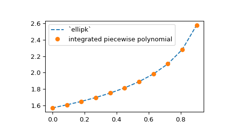
All piecewise polynomials can be constructed with N-dimensional y values. If y.ndim > 1, it is understood as a stack of 1D y values, which are arranged along the interpolation axis (with the default value of 0). The latter is specified via the axis argument, and the invariant is that len(x) == y.shape[axis]. As an example, we extend the elliptic integral example above to compute the approximation for a range of m values, using the NumPy broadcasting:

>>> from scipy.interpolate import PchipInterpolator
>>> m = np.linspace(0, 0.9, 11)
>>> x = np.linspace(0, np.pi/2, 70)
>>> y = 1 / np.sqrt(1 - m[:, None]*np.sin(x)**2)

Now the y array has the shape (11, 70), so that the values of y for fixed value of m are along the second axis of the y array.

>>> spl = PchipInterpolator(x, y, axis=1)  # the default is axis=0
>>> import matplotlib.pyplot as plt
>>> plt.plot(m, spl.integrate(0, np.pi/2), '--')

>>> from scipy.special import ellipk
>>> plt.plot(m, ellipk(m), 'o')
>>> plt.legend(['`ellipk`', 'integrated piecewise polynomial'])
>>> plt.show()

B-splines: knots and coefficients

A b-spline function — for instance, constructed from data via a make_interp_spline call — is defined by the so-called knots and coefficients.

As an illustration, let us again construct the interpolation of a sine function. The knots are available as the t attribute of a BSpline instance:

>>> x = np.linspace(0, 3/2, 7)
>>> y = np.sin(np.pi*x)
>>> from scipy.interpolate import make_interp_spline
>>> bspl = make_interp_spline(x, y, k=3)
>>> print(bspl.t)
[0.  0.  0.  0.        0.5  0.75  1.        1.5  1.5  1.5  1.5 ]
>>> print(x)
[            0.  0.25  0.5  0.75  1.  1.25  1.5 ]

We see that the knot vector by default is constructed from the input array x: first, it is made \((k+1)\) -regular (it has k repeated knots appended and prepended); then, the second and second-to-last points of the input array are removed—this is the so-called not-a-knot boundary condition.

In general, an interpolating spline of degree k needs len(t) - len(x) - k - 1 boundary conditions. For cubic splines with (k+1)-regular knot arrays this means two boundary conditions—or removing two values from the x array. Various boundary conditions can be requested using the optional bc_type argument of make_interp_spline.

The b-spline coefficients are accessed via the c attribute of a BSpline object:

>>> len(bspl.c)
7

The convention is that for len(t) knots there are len(t) - k - 1 coefficients. Some routines (see the Smoothing splines section) zero-pad the c arrays so that len(c) == len(t). These additional coefficients are ignored for evaluation.

We stress that the coefficients are given in the b-spline basis, not the power basis of \(1, x, \cdots, x^k\).

B-spline basis elements

The b-spline basis is used in a variety of applications which include interpolation, regression and curve representation. B-splines are piecewise polynomials, represented as linear combinations of b-spline basis elements — which themselves are certain linear combinations of usual monomials, \(x^m\) with \(m=0, 1, \dots, k\).

The properties of b-splines are well described in the literature (see, for example, references listed in the BSpline docstring). For our purposes, it is enough to know that a b-spline function is uniquely defined by an array of coefficients and an array of the so-called knots, which may or may not coincide with the data points, x.

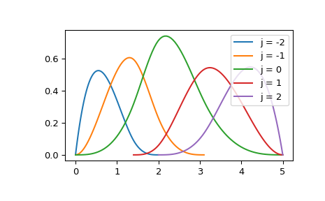
Specifically, a b-spline basis element of degree k (e.g. k=3 for cubics) is defined by \(k+2\) knots and is zero outside of these knots. To illustrate, plot a collection of non-zero basis elements on a certain interval:

>>> k = 3      # cubic splines
>>> t = [0., 1.4, 2., 3.1, 5.]   # internal knots
>>> t = np.r_[[0]*k, t, [5]*k]   # add boundary knots

>>> from scipy.interpolate import BSpline
>>> import matplotlib.pyplot as plt
>>> for j in [-2, -1, 0, 1, 2]:
...     a, b = t[k+j], t[-k+j-1]
...     xx = np.linspace(a, b, 101)
...     bspl = BSpline.basis_element(t[k+j:-k+j])
...     plt.plot(xx, bspl(xx), label=f'j = {j}')
>>> plt.legend(loc='best')
>>> plt.show()

Here BSpline.basis_element is essentially a shorthand for constructing a spline with only a single non-zero coefficient. For instance, the j=2 element in the above example is equivalent to

>>> c = np.zeros(t.size - k - 1)
>>> c[-2] = 1
>>> b = BSpline(t, c, k)
>>> np.allclose(b(xx), bspl(xx))
True

If desired, a b-spline can be converted into a PPoly object using PPoly.from_spline method which accepts a BSpline instance and returns a PPoly instance. The reverse conversion is performed by the BSpline.from_power_basis method. However, conversions between bases is best avoided because it accumulates rounding errors.

Design matrices in the B-spline basis

One common application of b-splines is in non-parametric regression. The reason is that the localized nature of the b-spline basis elements makes linear algebra banded. This is because at most \(k+1\) basis elements are non-zero at a given evaluation point, thus a design matrix built on b-splines has at most \(k+1\) diagonals.

As an illustration, we consider a toy example. Suppose our data are one-dimensional and are confined to an interval \([0, 6]\). We construct a 4-regular knot vector which corresponds to 7 data points and cubic, k=3, splines:

>>> t = [0., 0., 0., 0., 2., 3., 4., 6., 6., 6., 6.]

Next, take ‘observations’ to be

>>> xnew = [1, 2, 3]

and construct the design matrix in the sparse CSR format

>>> from scipy.interpolate import BSpline
>>> mat = BSpline.design_matrix(xnew, t, k=3)
>>> mat
<Compressed Sparse Row sparse array of dtype 'float64'
        with 12 stored elements and shape (3, 7)>

Here each row of the design matrix corresponds to a value in the xnew array, and a row has no more than k+1 = 4 non-zero elements; row j contains basis elements evaluated at xnew[j]:

>>> with np.printoptions(precision=3):
...     print(mat.toarray())
[[0.125 0.514 0.319 0.042 0.    0.    0.   ]
 [0.    0.111 0.556 0.333 0.    0.    0.   ]
 [0.    0.    0.125 0.75  0.125 0.    0.   ]]

Bernstein polynomials, BPoly

For \(t \in [0, 1]\), Bernstein basis polynomials of degree \(k\) are defined via

\[b(t; k, a) = C_k^a t^a (1-t)^{k - a}\]

where \(C_k^a\) is the binomial coefficient, and \(a=0, 1, \dots, k\), so that there are \(k+1\) basis polynomials of degree \(k\).

A BPoly object represents a piecewise Bernstein polynomial in terms of breakpoints, x, and coefficients, c: c[a, j] gives the coefficient for \(b(t; k, a)\) for t on the interval between x[j] and x[j+1].

The user interface of BPoly objects is very similar to that of PPoly objects: both can be evaluated, differentiated and integrated.

One additional feature of BPoly objects is the alternative constructor, BPoly.from_derivatives, which constructs a BPoly object from data values and derivatives. Specifically, b = BPoly.from_derivatives(x, y) returns a callable that interpolates the provided values, b(x[i]) == y[i]), and has the provided derivatives, b(x[i], nu=j) == y[i][j].

This operation is similar to CubicHermiteSpline, but it is more flexible in that it can handle varying numbers of derivatives at different data points; i.e., the y argument can be a list of arrays of different lengths. See BPoly.from_derivatives for further discussion and examples.

Conversion between bases

In principle, all three bases for piecewise polynomials (the power basis, the Bernstein basis, and b-splines) are equivalent, and a polynomial in one basis can be converted into a different basis. One reason for converting between bases is that not all bases implement all operations. For instance, root-finding is only implemented for PPoly, and therefore to find roots of a BSpline object, you need to convert to PPoly first. See methods PPoly.from_bernstein_basis, PPoly.from_spline, BPoly.from_power_basis, and BSpline.from_power_basis for details about conversion.

In floating-point arithmetic, though, conversions always incur some precision loss. Whether this is significant is problem-dependent, so it is therefore recommended to exercise caution when converting between bases.