1-D interpolation#
Piecewise linear interpolation#
If all you need is a linear (a.k.a. broken line) interpolation, you can use
the numpy.interp routine. It takes two arrays of data to interpolate, x,
and y, and a third array, xnew, of points to evaluate the interpolation on:
>>> import numpy as np
>>> x = np.linspace(0, 10, num=11)
>>> y = np.cos(-x**2 / 9.0)
Construct the interpolation
>>> xnew = np.linspace(0, 10, num=1001)
>>> ynew = np.interp(xnew, x, y)
And plot it
>>> import matplotlib.pyplot as plt
>>> plt.plot(xnew, ynew, '-', label='linear interp')
>>> plt.plot(x, y, 'o', label='data')
>>> plt.legend(loc='best')
>>> plt.show()

One limitation of numpy.interp is that it does not allow controlling the
extrapolation. See the interpolation with B-Splines section
section for alternative routines which provide this kind of functionality.
Cubic splines#
Of course, piecewise linear interpolation produces corners at data points,
where the linear pieces join. To produce a smoother curve, you can use cubic
splines, where the interpolating curve is made of cubic pieces with matching
first and second derivatives. In code, these objects are represented by instances of the
CubicSpline class. An instance is constructed with the x and
y arrays of data, and then it can be evaluated using the target xnew
values:
>>> from scipy.interpolate import CubicSpline
>>> spl = CubicSpline([1, 2, 3, 4, 5, 6], [1, 4, 8, 16, 25, 36])
>>> spl(2.5)
5.57
A CubicSpline object’s __call__ method accepts both scalar values and
arrays. It also accepts a second argument, nu, to evaluate the
derivative of order nu. As an example, we plot the derivatives of a spline:
>>> from scipy.interpolate import CubicSpline
>>> x = np.linspace(0, 10, num=11)
>>> y = np.cos(-x**2 / 9.)
>>> spl = CubicSpline(x, y)
>>> import matplotlib.pyplot as plt
>>> fig, ax = plt.subplots(4, 1, figsize=(5, 7))
>>> xnew = np.linspace(0, 10, num=1001)
>>> ax[0].plot(xnew, spl(xnew))
>>> ax[0].plot(x, y, 'o', label='data')
>>> ax[1].plot(xnew, spl(xnew, nu=1), '--', label='1st derivative')
>>> ax[2].plot(xnew, spl(xnew, nu=2), '--', label='2nd derivative')
>>> ax[3].plot(xnew, spl(xnew, nu=3), '--', label='3rd derivative')
>>> for j in range(4):
...     ax[j].legend(loc='best')
>>> plt.tight_layout()
>>> plt.show()
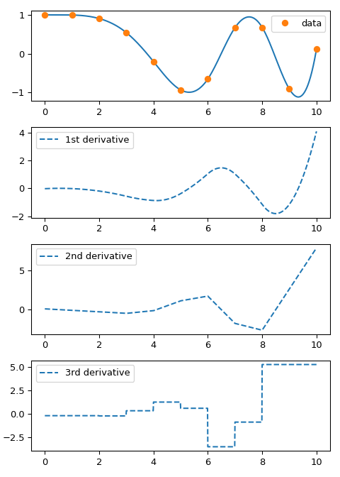
Note that the first and second derivatives are continuous by construction, and the third derivative jumps at data points.
Monotone interpolants#
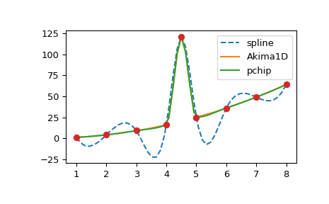
Cubic splines are by construction twice continuously differentiable. This may
lead to the spline function oscillating and ‘’overshooting’’ in between the
data points. In these situations, an alternative is to use the so-called
monotone cubic interpolants: these are constructed to be only once
continuously differentiable, and attempt to preserve the local shape implied
by the data. scipy.interpolate provides two objects of this kind:
PchipInterpolator and Akima1DInterpolator. To illustrate, let’s consider
data with an outlier:
>>> from scipy.interpolate import CubicSpline, PchipInterpolator, Akima1DInterpolator
>>> x = np.array([1., 2., 3., 4., 4.5, 5., 6., 7., 8])
>>> y = x**2
>>> y[4] += 101
>>> import matplotlib.pyplot as plt
>>> xx = np.linspace(1, 8, 51)
>>> plt.plot(xx, CubicSpline(x, y)(xx), '--', label='spline')
>>> plt.plot(xx, Akima1DInterpolator(x, y)(xx), '-', label='Akima1D')
>>> plt.plot(xx, PchipInterpolator(x, y)(xx), '-', label='pchip')
>>> plt.plot(x, y, 'o')
>>> plt.legend()
>>> plt.show()
Interpolation with B-splines#
B-splines form an alternative (though formally equivalent) representation of piecewise polynomials. This basis is generally more computationally stable than the power basis and is useful for a variety of applications which include interpolation, regression and curve representation. Details are given in the piecewise polynomials section, and here we illustrate their usage by constructing the interpolation of a sine function:
>>> x = np.linspace(0, 3/2, 7)
>>> y = np.sin(np.pi*x)
To construct the interpolating objects given data arrays, x and y,
we use the make_interp_spline function:
>>> from scipy.interpolate import make_interp_spline
>>> bspl = make_interp_spline(x, y, k=3)
This function returns an object which has an interface similar to that
of the CubicSpline objects. In particular, it can be evaluated at a data
point and differentiated:
>>> der = bspl.derivative()      # a BSpline representing the derivative
>>> import matplotlib.pyplot as plt
>>> xx = np.linspace(0, 3/2, 51)
>>> plt.plot(xx, bspl(xx), '--', label=r'$\sin(\pi x)$ approx')
>>> plt.plot(x, y, 'o', label='data')
>>> plt.plot(xx, der(xx)/np.pi, '--', label=r'$d \sin(\pi x)/dx / \pi$ approx')
>>> plt.legend()
>>> plt.show()
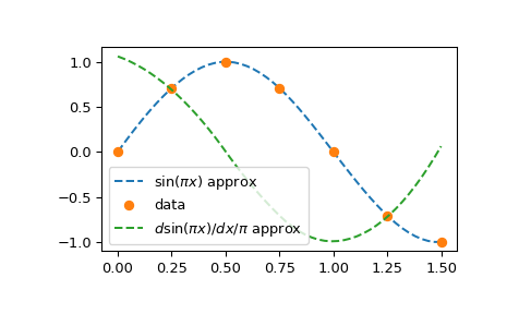
Note that by specifying k=3 in the make_interp_spline call, we requested
a cubic spline (this is the default, so k=3 could have been omitted); the
derivative of a cubic is a quadratic:
>>> bspl.k, der.k
(3, 2)
By default, the result of make_interp_spline(x, y) is equivalent to
CubicSpline(x, y). The difference is that the former allows several optional
capabilities: it can construct splines of various degrees (via the optional
argument k) and predefined knots (via the optional argument t).
Boundary conditions for the spline interpolation can be controlled by
the bc_type argument to make_interp_spline function and CubicSpline
constructor. By default, both use the ‘not-a-knot’ boundary
condition.
Non-cubic splines#
One use of make_interp_spline is constructing a linear interpolant with
linear extrapolation since make_interp_spline extrapolates by default. Consider
>>> from scipy.interpolate import make_interp_spline
>>> x = np.linspace(0, 5, 11)
>>> y = 2*x
>>> spl = make_interp_spline(x, y, k=1)  # k=1: linear
>>> spl([-1, 6])
[-2., 12.]
>>> np.interp([-1, 6], x, y)
[0., 10.]
See the extrapolation section for more details and discussion.
Batches of y#
Univariate interpolators accept not only one-dimensional y arrays, but also
y.ndim > 1. The interpretation is that y is a batch of 1D data arrays: by
default, the zeroth dimension of y is the interpolation axis, and the trailing
dimensions are batch dimensions.
Consider a collection (a batch) of functions \(f_j\) sampled at the points
\(x_i\). We can instantiate a single interpolator for all of these functions by
providing a two-dimensional array y such that y[i, j] records \(f_j(x_i)\).
To illustrate:
>>> import numpy as np
>>> import matplotlib.pyplot as plt
>>> from scipy.interpolate import make_interp_spline
>>> n = 11
>>> x = 2 * np.pi * np.arange(n) / n
>>> x.shape
(11,)
>>> y = np.stack((np.sin(x)**2, np.cos(x)), axis=1)
>>> y.shape
(11, 2)
>>> spl = make_interp_spline(x, y)
>>> xv = np.linspace(0, 2*np.pi, 51)
>>> plt.plot(x, y, 'o')
>>> plt.plot(xv, spl(xv), '-')
>>> plt.show()
Several notes are in order. First and foremost, the behavior here looks similar to NumPy’s broadcasting, but differs in two respects:
The
xarray is expected to be 1D even if theyarray is not:x.ndim == 1whiley.ndim >= 1. There is no broadcasting ofxvsy.By default, the trailing dimensions are used as batch dimensions, in contrast to the NumPy convention of using the leading dimensions as batch dimensions.
Second, the interpolation axis can be controlled by an optional axis argument. The
example above uses the default value of axis=0. For a non-default values, the
following is true:
y.shape[axis] == x.size(otherwise an error is raised)the shape of
spl(xv)isy.shape[axis:] + xv.shape + y.shape[:axis]
While we demonstrated the batching behavior with make_interp_spline, in fact the
majority of univariate interpolators support this functionality: PchipInterpolator and
Akima1DInterpolator, CubicSpline; low-level polynomial representation classes,
PPoly, BPoly and BSpline; as well as least-squares fit and spline smoothing
functions, make_lsq_spline and make_smoothing_spline.
Parametric spline curves#
So far we considered spline functions, where the data, y, is expected to
depend explicitly on the independent variable x—so that the interpolating
function satisfies \(f(x_j) = y_j\). Spline curves treat
the x and y arrays as coordinates of points, \(\mathbf{p}_j\) on a
plane, and an interpolating curve which passes through these points is
parameterized by some additional parameter (typically called u). Note that
this construction readily generalizes to higher dimensions where
\(\mathbf{p}_j\) are points in an N-dimensional space.
Spline curves can be easily constructed using the fact that interpolation
functions handle multidimensional data arrays, as discussed in
the previous section.
The values of the parameter, u, corresponding to the data points, need to be
separately supplied by the user.
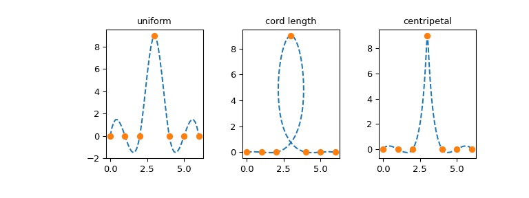
The choice of parametrization is problem-dependent and different parametrizations
may produce vastly different curves. As an example, we consider three
parametrizations of (a somewhat difficult) dataset, which we take from
Chapter 6 of Ref [1] listed in the BSpline docstring:
>>> x = [0, 1, 2, 3, 4, 5, 6]
>>> y = [0, 0, 0, 9, 0, 0, 0]
>>> p = np.stack((x, y))
>>> p
array([[0, 1, 2, 3, 4, 5, 6],
       [0, 0, 0, 9, 0, 0, 0]])
We take elements of the p array as coordinates of seven points on the
plane, where p[:, j] gives the coordinates of the point
\(\mathbf{p}_j\).
First, consider the uniform parametrization, \(u_j = j\):
>>> u_unif = x
Second, we consider the so-called chord length parametrization, which is nothing but a cumulative length of straight line segments connecting the data points:
for \(j=1, 2, \dots\) and \(u_0 = 0\). Here \(| \cdots |\) is the length between the consecutive points \(p_j\) on the plane.
>>> dp = p[:, 1:] - p[:, :-1]      # 2-vector distances between points
>>> l = (dp**2).sum(axis=0)        # squares of lengths of 2-vectors between points
>>> u_chord = np.sqrt(l).cumsum()   # cumulative sums of 2-norms
>>> u_chord = np.r_[0, u_chord]      # the first point is parameterized at zero
Finally, we consider what is sometimes called the centripetal parametrization: \(u_j = u_{j-1} + |\mathbf{p}_j - \mathbf{p}_{j-1}|^{1/2}\). Due to the extra square root, the difference between consecutive values \(u_j - u_{j-1}\) will be smaller than for the chord length parametrization:
>>> u_c = np.r_[0, np.cumsum((dp**2).sum(axis=0)**0.25)]
Now plot the resulting curves:
>>> from scipy.interpolate import make_interp_spline
>>> import matplotlib.pyplot as plt
>>> fig, ax = plt.subplots(1, 3, figsize=(8, 3))
>>> parametrizations = ['uniform', 'chord length', 'centripetal']
>>>
>>> for j, u in enumerate([u_unif, u_chord, u_c]):
...    spl = make_interp_spline(u, p, axis=1)    # note p is a 2D array
...
...    uu = np.linspace(u[0], u[-1], 51)
...    xx, yy = spl(uu)
...
...    ax[j].plot(xx, yy, '--')
...    ax[j].plot(p[0, :], p[1, :], 'o')
...    ax[j].set_title(parametrizations[j])
>>> plt.show()
Missing data#
We note that scipy.interpolate does not support interpolation with missing
data. Two popular ways of representing missing data are using masked arrays of
the numpy.ma library, and encoding missing values as not-a-number, NaN.
Neither of these two approaches is directly supported in scipy.interpolate.
Individual routines may offer partial support, and/or workarounds, but in
general, the library firmly adheres to the IEEE 754 semantics where a NaN
means not-a-number, i.e. a result of an illegal mathematical operation
(e.g., division by zero), not missing.
Out-of-bounds behavior#
Several interpolators in scipy.interpolate share a common way to control the
out-of-bounds behavior, including CubicSpline, CubicHermiteSpline,
Akima1DInterpolator, PchipInterpolator, PPoly,
BPoly, and BSpline.
There are two principal ingredients which affect the out-of-bounds behavior:
bc_type and extrapolate arguments. The former controls how the object
is constructed, and the latter controls how it is evaluated.
The bc_type parameter#
For CubicSpline and make_interp_spline, the bc_type
construction-time argument controls the shape of the spline at its boundaries and
therefore also affects extrapolation. When bc_type="periodic", periodic boundary
conditions are enforced and the interpolant is smooth at the join point. For all other
values of bc_type, out-of-bounds behavior is controlled separately by the
extrapolate argument described below.
To illustrate, we compare several values of the extrapolate constructor argument
for CubicSpline, including bc_type="periodic" which produces a smooth
periodic interpolant:
import matplotlib.pyplot as plt
import numpy as np
from scipy.interpolate import CubicSpline

# data
x = np.array([0, 1, 2.5, 3, 4])
y = np.array([0.0, 1.0, 0.8, 1.2, 0.0])
# evaluation points
x_eval = np.linspace(-4, 8, 300)

fig, ax = plt.subplots(figsize=(8, 6))
for extrapolate, linestyle in zip(
    [True, False, "periodic"], ["-", "--", ":"], strict=True
):
    y_interp = CubicSpline(x, y, extrapolate=extrapolate)(x_eval)
    ax.plot(x_eval, y_interp, linestyle, label=f"extrapolate={extrapolate}")

ax.plot(
    x_eval,
    CubicSpline(x, y, bc_type="periodic")(x_eval),
    "-.",
    label="bc_type='periodic'",
)
ax.plot(x, y, "ko", label="data")
ax.axvline(x[0] - 4, color="k", alpha=0.2)
ax.axvline(x[0], color="k", alpha=0.2)
ax.axvline(x[-1], color="k", alpha=0.2)
ax.axvline(x[-1] + 4, color="k", alpha=0.2)
ax.set_ylim(-0.5, 1.5)
ax.legend(ncol=2, loc="lower left")
ax.set_xlabel("x")
ax.set_ylabel("f(x)")
ax.set_title("CubicSpline")
plt.show()

Note that using bc_type="periodic" (red curve) enforces equal derivatives at the
boundaries of the interpolation interval (x=0 and x=4), so that the resulting
interpolant extends smoothly as a periodic function.
On the contrary, using extrapolate="periodic" together with the default value for bc_type (the green curve) does not enforce any boundary conditions, and simply extends the interpolant
+ periodically outside the data domain. See CubicSpline extend the boundary conditions for an additional discussion of how different bc_type values affect the interpolant.
The extrapolate constructor argument#
All the interpolators listed above accept an extrapolate keyword at construction
time, which sets the default out-of-bounds behavior for all subsequent evaluations:
extrapolate=True(default for most): evaluate the boundary polynomial pieces;extrapolate=False: returnNaN;extrapolate="periodic"(if supported): wrap the evaluation periodically.
The default is True for most interpolators, with two exceptions:
Akima1DInterpolator defaults to False, and bc_type="periodic"
forces the default to extrapolate="periodic".
To illustrate, we consider PchipInterpolator with several values of the
extrapolate constructor argument:
import matplotlib.pyplot as plt
import numpy as np
from scipy.interpolate import PchipInterpolator

# data
x = np.array([0, 1, 2.5, 3, 4])
y = np.array([0.0, 1.0, 0.8, 1.2, 0.0])
# evaluation points
x_eval = np.linspace(-4, 8, 300)

fig, ax = plt.subplots(figsize=(8, 6))
for extrapolate, linestyle in zip(
    [True, False, "periodic"], ["-", "--", ":"], strict=True
):
    y_interp = PchipInterpolator(x, y, extrapolate=extrapolate)(x_eval)
    ax.plot(x_eval, y_interp, linestyle, label=f"extrapolate={extrapolate}")
ax.plot(x, y, "k.", markersize=8, label="data")
ax.axvline(x[0] - 4, color="k", alpha=0.2)
ax.axvline(x[0], color="k", alpha=0.2)
ax.axvline(x[-1], color="k", alpha=0.2)
ax.axvline(x[-1] + 4, color="k", alpha=0.2)
ax.set_ylim(-2.0, 2.5)
ax.legend(ncol=2, loc="lower left")
ax.set_xlabel("x")
ax.set_ylabel("f(x)")
ax.set_title("PchipInterpolator")
plt.show()

Note that PchipInterpolator has no bc_type argument, so there is
no way to construct a truly periodic PCHIP interpolant. Using
extrapolate="periodic" only wraps evaluation at the domain boundaries
and makes no guarantees about smoothness at the join point, as visible in
the plot above.
Overriding extrapolate per call#
The extrapolate argument can also be passed at evaluation time (i.e. when
calling the interpolator object). Passing extrapolate=None (the default) means
“use the value that was set at construction time.” Passing any other value
overrides the construction-time setting for that call only:
>>> from scipy.interpolate import CubicSpline
>>> import numpy as np
>>> spl = CubicSpline([0, 1, 2], [0, 1, 0], extrapolate=False)
>>> x_eval = np.array([-1, 0.5, 3])
>>> spl(x_eval)           # uses construction-time extrapolate=False
array([nan, 0.75, nan])
>>> spl(x_eval, extrapolate=True)   # override for this call
array([-3.,  0.75,  -3.])
See Extrapolation tips and tricks for further details.
Legacy interface for 1-D interpolation (interp1d)#
Note
interp1d is considered legacy API and is not recommended for use in new
code. Consider using more specific interpolators instead.
The interp1d class in scipy.interpolate is a convenient method to
create a function based on fixed data points, which can be evaluated
anywhere within the domain defined by the given data using linear
interpolation. An instance of this class is created by passing the 1-D
vectors comprising the data. The instance of this class defines a
__call__ method and can therefore be treated like a function which
interpolates between known data values to obtain unknown values.
Behavior at the boundary can be
specified at instantiation time. The following example demonstrates
its use, for linear and cubic spline interpolation:
>>> from scipy.interpolate import interp1d
>>> x = np.linspace(0, 10, num=11, endpoint=True)
>>> y = np.cos(-x**2/9.0)
>>> f = interp1d(x, y)
>>> f2 = interp1d(x, y, kind='cubic')
>>> xnew = np.linspace(0, 10, num=41, endpoint=True)
>>> import matplotlib.pyplot as plt
>>> plt.plot(x, y, 'o', xnew, f(xnew), '-', xnew, f2(xnew), '--')
>>> plt.legend(['data', 'linear', 'cubic'], loc='best')
>>> plt.show()
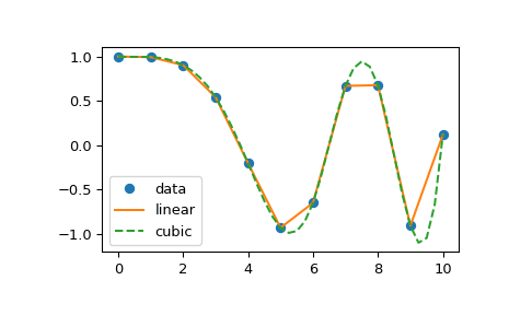
The ‘cubic’ kind of interp1d is equivalent to make_interp_spline, and
the ‘linear’ kind is equivalent to numpy.interp while also allowing
N-dimensional y arrays.
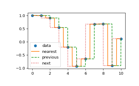
Another set of interpolations in interp1d is nearest, previous, and
next, where they return the nearest, previous, or next point along the
x-axis. Nearest and next can be thought of as a special case of a causal
interpolating filter. The following example demonstrates their use, using the
same data as in the previous example:
>>> from scipy.interpolate import interp1d
>>> x = np.linspace(0, 10, num=11, endpoint=True)
>>> y = np.cos(-x**2/9.0)
>>> f1 = interp1d(x, y, kind='nearest')
>>> f2 = interp1d(x, y, kind='previous')
>>> f3 = interp1d(x, y, kind='next')
>>> xnew = np.linspace(0, 10, num=1001, endpoint=True)
>>> import matplotlib.pyplot as plt
>>> plt.plot(x, y, 'o')
>>> plt.plot(xnew, f1(xnew), '-', xnew, f2(xnew), '--', xnew, f3(xnew), ':')
>>> plt.legend(['data', 'nearest', 'previous', 'next'], loc='best')
>>> plt.show()
Recommended replacements for interp1d modes#
As mentioned, interp1d class is legacy: we have no plans to remove it; we
are going to keep supporting its existing usages; however
we believe there are better alternatives which we recommend using in new code.
Here we list specific recommendations, depending on the interpolation kind.
Linear interpolation, kind="linear"
The default recommendation is to use numpy.interp function. Alternatively,
you can use linear splines, make_interp_spline(x, y, k=1), see
this section for a discussion.
Spline interpolators, kind="quadratic" or "cubic"
Under the hood, interp1d delegates to make_interp_spline, so we recommend
using the latter directly.
Piecewise constant modes, kind="nearest", "previous", "next"
First, we note that interp1d(x, y, kind='previous') is equivalent to
make_interp_spline(x, y, k=0).
More generally however, all these piecewise constant interpolation modes are
based on numpy.searchsorted. For example, the "nearest" mode is nothing but
>>> x = np.arange(8)
>>> y = x**2
>>> x_new = np.linspace(0, 7, 101)    # input points
>>> x_bds = x[:-1] / 2.0 + x[1:] / 2.0   # halfway points
>>> idx = np.searchsorted(x_bds, x_new, side='left')
>>> idx = np.clip(idx, 0, len(x) - 1)  # clip the indices so that they are within the range of x indices.
>>> import matplotlib.pyplot as plt
>>> plt.plot(x, y, 'o')
>>> plt.plot(x_new, y[idx], '--')
>>> plt.show()
Other variants are similar, see the interp1d source code
for details.