scipy.interpolate.

CubicSpline

class scipy.interpolate.CubicSpline(x, y, axis=0, bc_type='not-a-knot', extrapolate=None)

Piecewise cubic interpolator to fit values (C2 smooth).

Interpolate data with a piecewise cubic polynomial which is twice continuously differentiable [1]. The result is represented as a PPoly instance with breakpoints matching the given data.

Parameters:

xarray_like, shape (n,)

1-D array containing values of the independent variable. Values must be real, finite and in strictly increasing order.

yarray_like

Array containing values of the dependent variable. It can have arbitrary number of dimensions, but the length along axis (see below) must match the length of x. Values must be finite.

axisint, optional

Axis along which y is assumed to be varying. Meaning that for x[i] the corresponding values are np.take(y, i, axis=axis). Default is 0.

bc_typestring or 2-tuple, optional

Boundary condition type. Two additional equations, given by the boundary conditions, are required to determine all coefficients of polynomials on each segment [2].

If bc_type is a string, then the specified condition will be applied at both ends of a spline. Available conditions are:

• ‘not-a-knot’ (default): The first and second segment at a curve end are the same polynomial. It is a good default when there is no information on boundary conditions.

• ‘periodic’: The interpolated functions is assumed to be periodic of period x[-1] - x[0]. The first and last value of y must be identical: y[0] == y[-1]. This boundary condition will result in y'[0] == y'[-1] and y''[0] == y''[-1].

• ‘clamped’: The first derivative at curves ends are zero. Assuming a 1D y, bc_type=((1, 0.0), (1, 0.0)) is the same condition.

• ‘natural’: The second derivative at curve ends are zero. Assuming a 1D y, bc_type=((2, 0.0), (2, 0.0)) is the same condition.

If bc_type is a 2-tuple, the first and the second value will be applied at the curve start and end respectively. The tuple values can be one of the previously mentioned strings (except ‘periodic’) or a tuple (order, deriv_values) allowing to specify arbitrary derivatives at curve ends:

• order: the derivative order, 1 or 2.

• deriv_value: array_like containing derivative values, shape must be the same as y, excluding axis dimension. For example, if y is 1-D, then deriv_value must be a scalar. If y is 3-D with the shape (n0, n1, n2) and axis=2, then deriv_value must be 2-D and have the shape (n0, n1).

extrapolate{bool, ‘periodic’, None}, optional

If bool, determines whether to extrapolate to out-of-bounds points based on first and last intervals, or to return NaNs. If ‘periodic’, periodic extrapolation is used. If None (default), extrapolate is set to ‘periodic’ for bc_type='periodic' and to True otherwise.

Attributes:

xndarray, shape (n,)

Breakpoints. The same x which was passed to the constructor.

cndarray, shape (4, n-1, …)

Coefficients of the polynomials on each segment. The trailing dimensions match the dimensions of y, excluding axis. For example, if y is 1-d, then c[k, i] is a coefficient for (x-x[i])**(3-k) on the segment between x[i] and x[i+1].

axisint

Interpolation axis. The same axis which was passed to the constructor.

Methods

__call__(x[, nu, extrapolate])	Evaluate the piecewise polynomial or its derivative.
derivative([nu])	Construct a new piecewise polynomial representing the derivative.
antiderivative([nu])	Construct a new piecewise polynomial representing the antiderivative.
integrate(a, b[, extrapolate])	Compute a definite integral over a piecewise polynomial.
solve([y, discontinuity, extrapolate])	Find real solutions of the equation pp(x) == y.
roots([discontinuity, extrapolate])	Find real roots of the piecewise polynomial.

See also

Akima1DInterpolator

Akima 1D interpolator.

PchipInterpolator

PCHIP 1-D monotonic cubic interpolator.

PPoly

Piecewise polynomial in terms of coefficients and breakpoints.

Notes

Parameters bc_type and extrapolate work independently, i.e. the former controls only construction of a spline, and the latter only evaluation.

When a boundary condition is ‘not-a-knot’ and n = 2, it is replaced by a condition that the first derivative is equal to the linear interpolant slope. When both boundary conditions are ‘not-a-knot’ and n = 3, the solution is sought as a parabola passing through given points.

When ‘not-a-knot’ boundary conditions is applied to both ends, the resulting spline will be the same as returned by splrep (with s=0) and InterpolatedUnivariateSpline, but these two methods use a representation in B-spline basis.

Added in version 0.18.0.

Array API Standard Support

CubicSpline has experimental support for Python Array API Standard compatible backends in addition to NumPy. Please consider testing these features by setting an environment variable SCIPY_ARRAY_API=1 and providing CuPy, PyTorch, JAX, or Dask arrays as array arguments. The following combinations of backend and device (or other capability) are supported.

Library	CPU	GPU
NumPy	✅	n/a
CuPy	n/a	⛔
PyTorch	✅	⛔
JAX	⚠️ no JIT	⛔
Dask	⛔	n/a

See Support for the array API standard for more information.

References

[1]

Cubic Spline Interpolation on Wikiversity.

[2]

Carl de Boor, “A Practical Guide to Splines”, Springer-Verlag, 1978.

Examples

Try it in your browser!

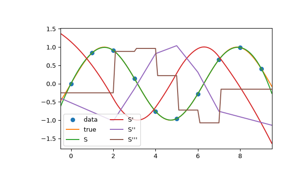
In this example the cubic spline is used to interpolate a sampled sinusoid. You can see that the spline continuity property holds for the first and second derivatives and violates only for the third derivative.

>>> import numpy as np
>>> from scipy.interpolate import CubicSpline
>>> import matplotlib.pyplot as plt
>>> x = np.arange(10)
>>> y = np.sin(x)
>>> cs = CubicSpline(x, y)
>>> xs = np.arange(-0.5, 9.6, 0.1)
>>> fig, ax = plt.subplots(figsize=(6.5, 4))
>>> ax.plot(x, y, 'o', label='data')
>>> ax.plot(xs, np.sin(xs), label='true')
>>> ax.plot(xs, cs(xs), label="S")
>>> ax.plot(xs, cs(xs, 1), label="S'")
>>> ax.plot(xs, cs(xs, 2), label="S''")
>>> ax.plot(xs, cs(xs, 3), label="S'''")
>>> ax.set_xlim(-0.5, 9.5)
>>> ax.legend(loc='lower left', ncol=2)
>>> plt.show()

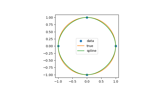
In the second example, the unit circle is interpolated with a spline. A periodic boundary condition is used. You can see that the first derivative values, ds/dx=0, ds/dy=1 at the periodic point (1, 0) are correctly computed. Note that a circle cannot be exactly represented by a cubic spline. To increase precision, more breakpoints would be required.

>>> theta = 2 * np.pi * np.linspace(0, 1, 5)
>>> y = np.c_[np.cos(theta), np.sin(theta)]
>>> cs = CubicSpline(theta, y, bc_type='periodic')
>>> print("ds/dx={:.1f} ds/dy={:.1f}".format(cs(0, 1)[0], cs(0, 1)[1]))
ds/dx=0.0 ds/dy=1.0
>>> xs = 2 * np.pi * np.linspace(0, 1, 100)
>>> fig, ax = plt.subplots(figsize=(6.5, 4))
>>> ax.plot(y[:, 0], y[:, 1], 'o', label='data')
>>> ax.plot(np.cos(xs), np.sin(xs), label='true')
>>> ax.plot(cs(xs)[:, 0], cs(xs)[:, 1], label='spline')
>>> ax.axes.set_aspect('equal')
>>> ax.legend(loc='center')
>>> plt.show()

The third example is the interpolation of a polynomial y = x**3 on the interval 0 <= x<= 1. A cubic spline can represent this function exactly. To achieve that we need to specify values and first derivatives at endpoints of the interval. Note that y’ = 3 * x**2 and thus y’(0) = 0 and y’(1) = 3.

>>> cs = CubicSpline([0, 1], [0, 1], bc_type=((1, 0), (1, 3)))
>>> x = np.linspace(0, 1)
>>> np.allclose(x**3, cs(x))
True

Go BackOpen In Tab