scipy.special.ellipk#

scipy.special.ellipk(m, out=None) = <ufunc 'ellipk'>#

Complete elliptic integral of the first kind.

This function is defined as

\[K(m) = \int_0^{\pi/2} [1 - m \sin(t)^2]^{-1/2} dt\]

Parameters:

marray_like: The parameter of the elliptic integral.
outndarray, optional: Optional output array for the function values

Returns:

Kscalar or ndarray: Value of the elliptic integral.

See also

ellipkm1: Complete elliptic integral of the first kind around m = 1
ellipkinc: Incomplete elliptic integral of the first kind
ellipe: Complete elliptic integral of the second kind
ellipeinc: Incomplete elliptic integral of the second kind
elliprf: Completely-symmetric elliptic integral of the first kind.

Notes

For more precision around point m = 1, use ellipkm1, which this function calls.

The parameterization in terms of \(m\) follows that of section 17.2 in [1]. Other parameterizations in terms of the complementary parameter \(1 - m\), modular angle \(\sin^2(\alpha) = m\), or modulus \(k^2 = m\) are also used, so be careful that you choose the correct parameter.

The Legendre K integral is related to Carlson’s symmetric R_F function by [2]:

\[K(m) = R_F(0, 1-k^2, 1) .\]

Array API Standard Support

ellipk has experimental support for Python Array API Standard compatible backends in addition to NumPy. Please consider testing these features by setting an environment variable SCIPY_ARRAY_API=1 and providing CuPy, PyTorch, JAX, or Dask arrays as array arguments. The following combinations of backend and device (or other capability) are supported.

Library	CPU	GPU
NumPy	✅	n/a
CuPy	n/a	✅
PyTorch	✅	⛔
JAX	✅	⛔
Dask	✅	n/a

See Support for the array API standard for more information.

References

[1]

Milton Abramowitz and Irene A. Stegun, eds. Handbook of Mathematical Functions with Formulas, Graphs, and Mathematical Tables. New York: Dover, 1972.

[2]

NIST Digital Library of Mathematical Functions. http://dlmf.nist.gov/, Release 1.0.28 of 2020-09-15. See Sec. 19.25(i) https://dlmf.nist.gov/19.25#i

Examples

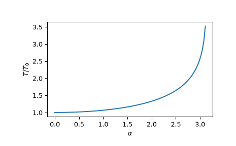
The period \(T\) of a simple pendulum increases with growing oscillation amplitude and can be expressed through the complete elliptic integral of the first kind. The plot displays the ratio of the period of the pendulum and the period \(T_0\) for small amplitude as a function of the maximum angle \(\alpha\) reached by the pendulum.

>>> import matplotlib.pyplot as plt
>>> import numpy as np
>>> from scipy.special import ellipk
>>> alpha = np.linspace(0, np.pi, 100)
>>> m = np.sin(alpha/2)**2
>>> fig, ax = plt.subplots()
>>> ax.plot(alpha, ellipk(m)*2/np.pi)
>>> ax.set_xlabel(r'$\alpha$')
>>> ax.set_ylabel('$T/T_0$')
>>> plt.show()

../../_images/scipy-special-ellipk-1.png