gaussian#
- scipy.signal.windows.gaussian(M, std, sym=True, *, xp=None, device=None)[source]#
Return a Gaussian window.
- Parameters:
- Mint
Number of points in the output window. If zero, an empty array is returned. An exception is thrown when it is negative.
- stdfloat
The standard deviation, sigma.
- symbool, optional
When True (default), generates a symmetric window, for use in filter design. When False, generates a periodic window, for use in spectral analysis.
- xparray_namespace, optional
Optional array namespace. Should be compatible with the array API standard, or supported by array-api-compat. Default:
numpy- deviceany
optional device specification for output. Should match one of the supported device specification in
xp.
- Returns:
- wndarray
The window, with the maximum value normalized to 1 (though the value 1 does not appear if M is even and sym is True).
Notes
The Gaussian window is defined as
\[w(n) = e^{ -\frac{1}{2}\left(\frac{n}{\sigma}\right)^2 }\]Array API Standard Support
gaussianhas experimental support for Python Array API Standard compatible backends in addition to NumPy. Please consider testing these features by setting an environment variableSCIPY_ARRAY_API=1and providing CuPy, PyTorch, JAX, or Dask arrays as array arguments. The following combinations of backend and device (or other capability) are supported.Library
CPU
GPU
NumPy
✅
n/a
CuPy
n/a
✅
PyTorch
✅
✅
JAX
✅
✅
Dask
✅
n/a
See Support for the array API standard for more information.
Examples
Plot the window and its frequency response:
>>> import numpy as np
>>> from scipy import signal
>>> from scipy.fft import fft, fftshift
>>> import matplotlib.pyplot as plt
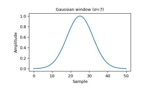
>>> window = signal.windows.gaussian(51, std=7)
>>> plt.plot(window)
>>> plt.title(r"Gaussian window ($\sigma$=7)")
>>> plt.ylabel("Amplitude")
>>> plt.xlabel("Sample")
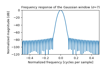
>>> plt.figure()
>>> A = fft(window, 2048) / (len(window)/2.0)
>>> freq = np.linspace(-0.5, 0.5, len(A))
>>> response = 20 * np.log10(np.abs(fftshift(A / abs(A).max())))
>>> plt.plot(freq, response)
>>> plt.axis([-0.5, 0.5, -120, 0])
>>> plt.title(r"Frequency response of the Gaussian window ($\sigma$=7)")
>>> plt.ylabel("Normalized magnitude [dB]")
>>> plt.xlabel("Normalized frequency [cycles per sample]")