scipy.signal.windows.

general_cosine

scipy.signal.windows.general_cosine(M, a, sym=True)

Generic weighted sum of cosine terms window

Parameters:

Mint

Number of points in the output window

aarray_like

Sequence of weighting coefficients. This uses the convention of being centered on the origin, so these will typically all be positive numbers, not alternating sign.

symbool, optional

When True (default), generates a symmetric window, for use in filter design. When False, generates a periodic window, for use in spectral analysis.

Returns:

wndarray

The array of window values.

Notes

Array API Standard Support

general_cosine has experimental support for Python Array API Standard compatible backends in addition to NumPy. Please consider testing these features by setting an environment variable SCIPY_ARRAY_API=1 and providing CuPy, PyTorch, JAX, or Dask arrays as array arguments. The following combinations of backend and device (or other capability) are supported.

Library	CPU	GPU
NumPy	✅	n/a
CuPy	n/a	✅
PyTorch	✅	✅
JAX	✅	✅
Dask	✅	n/a

See Support for the array API standard for more information.

References

[1]

A. Nuttall, “Some windows with very good sidelobe behavior,” IEEE Transactions on Acoustics, Speech, and Signal Processing, vol. 29, no. 1, pp. 84-91, Feb 1981. DOI:10.1109/TASSP.1981.1163506.

[2]

Heinzel G. et al., “Spectrum and spectral density estimation by the Discrete Fourier transform (DFT), including a comprehensive list of window functions and some new flat-top windows”, February 15, 2002 https://holometer.fnal.gov/GH_FFT.pdf

Examples

Try it in your browser!

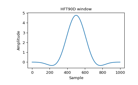
Heinzel describes a flat-top window named “HFT90D” with formula: [2]

\[w_j = 1 - 1.942604 \cos(z) + 1.340318 \cos(2z) - 0.440811 \cos(3z) + 0.043097 \cos(4z)\]

where

\[z = \frac{2 \pi j}{N}, j = 0...N - 1\]

Since this uses the convention of starting at the origin, to reproduce the window, we need to convert every other coefficient to a positive number:

>>> HFT90D = [1, 1.942604, 1.340318, 0.440811, 0.043097]

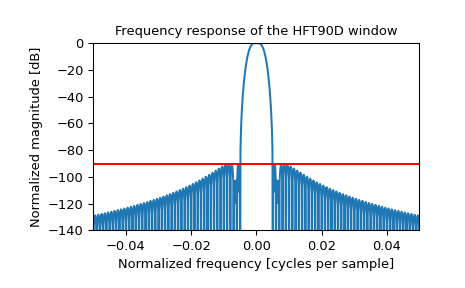
The paper states that the highest sidelobe is at -90.2 dB. Reproduce Figure 42 by plotting the window and its frequency response, and confirm the sidelobe level in red:

>>> import numpy as np
>>> from scipy.signal.windows import general_cosine
>>> from scipy.fft import fft, fftshift
>>> import matplotlib.pyplot as plt

>>> window = general_cosine(1000, HFT90D, sym=False)
>>> plt.plot(window)
>>> plt.title("HFT90D window")
>>> plt.ylabel("Amplitude")
>>> plt.xlabel("Sample")

>>> plt.figure()
>>> A = fft(window, 10000) / (len(window)/2.0)
>>> freq = np.linspace(-0.5, 0.5, len(A))
>>> response = np.abs(fftshift(A / abs(A).max()))
>>> response = 20 * np.log10(np.maximum(response, 1e-10))
>>> plt.plot(freq, response)
>>> plt.axis([-50/1000, 50/1000, -140, 0])
>>> plt.title("Frequency response of the HFT90D window")
>>> plt.ylabel("Normalized magnitude [dB]")
>>> plt.xlabel("Normalized frequency [cycles per sample]")
>>> plt.axhline(-90.2, color='red')
>>> plt.show()

Go BackOpen In Tab