scipy.signal.

freqs#

scipy.signal.freqs(b, a, worN=200, plot=None)[source]#

Compute frequency response of analog filter.

Given the M-order numerator b and N-order denominator a of an analog filter, compute its frequency response:

        b[0]*(jw)**M + b[1]*(jw)**(M-1) + ... + b[M]
H(w) = ----------------------------------------------
        a[0]*(jw)**N + a[1]*(jw)**(N-1) + ... + a[N]

Parameters:

barray_like: Numerator of a linear filter.
aarray_like: Denominator of a linear filter.
worN{None, int, array_like}, optional: If None, then compute at 200 frequencies around the interesting parts of the response curve (determined by pole-zero locations). If a single integer, then compute at that many frequencies. Otherwise, compute the response at the angular frequencies (e.g., rad/s) given in worN.
plotcallable, optional: A callable that takes two arguments. If given, the return parameters w and h are passed to plot. Useful for plotting the frequency response inside freqs.

Returns:

wndarray: The angular frequencies at which h was computed.
hndarray: The frequency response.

See also

freqz: Compute the frequency response of a digital filter.

Notes

Using Matplotlib’s “plot” function as the callable for plot produces unexpected results, this plots the real part of the complex transfer function, not the magnitude. Try lambda w, h: plot(w, abs(h)).

Array API Standard Support

freqs has experimental support for Python Array API Standard compatible backends in addition to NumPy. Please consider testing these features by setting an environment variable SCIPY_ARRAY_API=1 and providing CuPy, PyTorch, JAX, or Dask arrays as array arguments. The following combinations of backend and device (or other capability) are supported.

Library	CPU	GPU
NumPy	✅	n/a
CuPy	n/a	✅
PyTorch	✅	✅
JAX	⚠️ no JIT	⛔
Dask	⚠️ computes graph	n/a

See Support for the array API standard for more information.

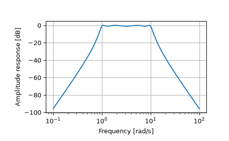
Examples

>>> from scipy.signal import freqs, iirfilter
>>> import numpy as np

>>> b, a = iirfilter(4, [1, 10], 1, 60, analog=True, ftype='cheby1')

>>> w, h = freqs(b, a, worN=np.logspace(-1, 2, 1000))

>>> import matplotlib.pyplot as plt
>>> plt.semilogx(w, 20 * np.log10(abs(h)))
>>> plt.xlabel('Frequency [rad/s]')
>>> plt.ylabel('Amplitude response [dB]')
>>> plt.grid(True)
>>> plt.show()