scipy.signal.

freqs_zpk#

scipy.signal.freqs_zpk(z, p, k, worN=200)[source]#

Compute frequency response of analog filter.

Given the zeros z, poles p, and gain k of a filter, compute its frequency response:

           (jw-z[0]) * (jw-z[1]) * ... * (jw-z[-1])
H(w) = k * ----------------------------------------
           (jw-p[0]) * (jw-p[1]) * ... * (jw-p[-1])

Parameters:

zarray_like: Zeroes of a linear filter
parray_like: Poles of a linear filter
kscalar: Gain of a linear filter
worN{None, int, array_like}, optional: If None, then compute at 200 frequencies around the interesting parts of the response curve (determined by pole-zero locations). If a single integer, then compute at that many frequencies. Otherwise, compute the response at the angular frequencies (e.g., rad/s) given in worN.

Returns:

wndarray: The angular frequencies at which h was computed.
hndarray: The frequency response.

See also

freqs: Compute the frequency response of an analog filter in TF form
freqz: Compute the frequency response of a digital filter in TF form
freqz_zpk: Compute the frequency response of a digital filter in ZPK form

Notes

Added in version 0.19.0.

Array API Standard Support

freqs_zpk has experimental support for Python Array API Standard compatible backends in addition to NumPy. Please consider testing these features by setting an environment variable SCIPY_ARRAY_API=1 and providing CuPy, PyTorch, JAX, or Dask arrays as array arguments. The following combinations of backend and device (or other capability) are supported.

Library	CPU	GPU
NumPy	✅	n/a
CuPy	n/a	✅
PyTorch	✅	✅
JAX	⚠️ no JIT	⛔
Dask	⚠️ computes graph	n/a

See Support for the array API standard for more information.

Examples

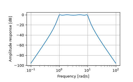
>>> import numpy as np
>>> from scipy.signal import freqs_zpk, iirfilter

>>> z, p, k = iirfilter(4, [1, 10], 1, 60, analog=True, ftype='cheby1',
...                     output='zpk')

>>> w, h = freqs_zpk(z, p, k, worN=np.logspace(-1, 2, 1000))

>>> import matplotlib.pyplot as plt
>>> plt.semilogx(w, 20 * np.log10(abs(h)))
>>> plt.xlabel('Frequency [rad/s]')
>>> plt.ylabel('Amplitude response [dB]')
>>> plt.grid(True)
>>> plt.show()

../../_images/scipy-signal-freqs_zpk-1.png