dfreqresp#
- scipy.signal.dfreqresp(system, w=None, n=10000, whole=False)[source]#
Calculate the frequency response of a discrete-time system.
- Parameters:
- systemdlti | tuple
An instance of the LTI class
dltior a tuple describing the system. The number of elements in the tuple determine the interpretation. I.e.:system: Instance of LTI classdlti. Note that derived instances, such as instances ofTransferFunction,ZerosPolesGain, orStateSpace, are allowed as well.(num, den, dt): Rational polynomial as described inTransferFunction. The coefficients of the polynomials should be specified in descending exponent order, e.g., z² + 3z + 5 would be represented as[1, 3, 5].(zeros, poles, gain, dt): Zeros, poles, gain form as described inZerosPolesGain.(A, B, C, D, dt): State-space form as described inStateSpace.
- warray_like, optional
Array of frequencies (in radians/sample). Magnitude and phase data is calculated for every value in this array. If not given a reasonable set will be calculated.
- nint, optional
Number of frequency points to compute if w is not given. The n frequencies are logarithmically spaced in an interval chosen to include the influence of the poles and zeros of the system.
- wholebool, optional
Normally, if ‘w’ is not given, frequencies are computed from 0 to the Nyquist frequency, pi radians/sample (upper-half of unit-circle). If whole is True, compute frequencies from 0 to 2*pi radians/sample.
- Returns:
- w1D ndarray
Frequency array [radians/sample]
- H1D ndarray
Array of complex magnitude values
Notes
If (num, den) is passed in for
system, coefficients for both the numerator and denominator should be specified in descending exponent order (e.g.z^2 + 3z + 5would be represented as[1, 3, 5]).Added in version 0.18.0.
Examples
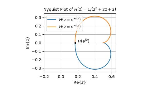
The following example generates the Nyquist plot of the transfer function \(H(z) = \frac{1}{z^2 + 2z + 3}\) with a sampling time of 0.05 seconds:
>>> from scipy import signal
>>> import matplotlib.pyplot as plt
>>> sys = signal.TransferFunction([1], [1, 2, 3], dt=0.05)  # construct H(z)
>>> w, H = signal.dfreqresp(sys)
...
>>> fig0, ax0 = plt.subplots()
>>> ax0.plot(H.real, H.imag, label=r"$H(z=e^{+j\omega})$")
>>> ax0.plot(H.real, -H.imag, label=r"$H(z=e^{-j\omega})$")
>>> ax0.set_title(r"Nyquist Plot of $H(z) = 1 / (z^2 + 2z + 3)$")
>>> ax0.set(xlabel=r"$\text{Re}\{z\}$", ylabel=r"$\text{Im}\{z\}$",
...         xlim=(-0.2, 0.65), aspect='equal')
>>> ax0.plot(H[0].real, H[0].imag, 'k.')  # mark H(exp(1j*w[0]))
>>> ax0.text(0.2, 0, r"$H(e^{j0})$")
>>> ax0.grid(True)
>>> ax0.legend()
>>> plt.show()