scipy.signal.

dstep#

scipy.signal.dstep(system, x0=None, t=None, n=None)[source]#

Step response of discrete-time system.

Parameters:

systemdlti | tuple

An instance of the LTI class dlti or a tuple describing the system. The number of elements in the tuple determine the interpretation. I.e.:

system: Instance of LTI class dlti. Note that derived instances, such as instances of TransferFunction, ZerosPolesGain, or StateSpace, are allowed as well.
(num, den, dt): Rational polynomial as described in TransferFunction. The coefficients of the polynomials should be specified in descending exponent order, e.g., z² + 3z + 5 would be represented as [1, 3, 5].
(zeros, poles, gain, dt): Zeros, poles, gain form as described in ZerosPolesGain.
(A, B, C, D, dt): State-space form as described in StateSpace.

x0array_like, optional

Initial state-vector. Defaults to zero.

tarray_like, optional

Time points. Computed if not given.

nint, optional

The number of time points to compute (if t is not given).

Returns:

toutndarray: Output time points, as a 1-D array.
youttuple of ndarray: Step response of system. Each element of the tuple represents the output of the system based on a step response to each input.

See also

step, dimpulse, dlsim, cont2discrete

Examples

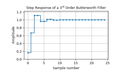
The following example illustrates how to create a digital Butterworth filer and plot its step response:

>>> import numpy as np
>>> from scipy import signal
>>> import matplotlib.pyplot as plt
...
>>> dt = 1  # sampling interval is one => time unit is sample number
>>> bb, aa = signal.butter(3, 0.25, fs=1/dt)
>>> t, y = signal.dstep((bb, aa, dt), n=25)
...
>>> fig0, ax0 = plt.subplots()
>>> ax0.step(t, np.squeeze(y), '.-', where='post')
>>> ax0.set_title(r"Step Response of a $3^\text{rd}$ Order Butterworth Filter")
>>> ax0.set(xlabel='Sample number', ylabel='Amplitude', ylim=(0, 1.1*np.max(y)))
>>> ax0.grid()
>>> plt.show()