scipy.interpolate.

RegularGridInterpolator

class scipy.interpolate.RegularGridInterpolator(points, values, method='linear', bounds_error=True, fill_value=nan, *, solver=None, solver_args=None)

Interpolator on a regular or rectilinear grid in arbitrary dimensions.

The data must be defined on a rectilinear grid; that is, a rectangular grid with even or uneven spacing. Linear, nearest-neighbor, spline interpolations are supported. After setting up the interpolator object, the interpolation method may be chosen at each evaluation.

Parameters:

pointstuple of ndarray of float, with shapes (m1, ), …, (mn, )

The points defining the regular grid in n dimensions. The points in each dimension (i.e. every elements of the points tuple) must be strictly ascending or descending.

valuesarray_like, shape (m1, …, mn, …)

The data on the regular grid in n dimensions. Complex data is accepted.

methodstr, optional

The method of interpolation to perform. Supported are “linear”, “nearest”, “slinear”, “cubic”, “quintic” and “pchip”. This parameter will become the default for the object’s __call__ method. Default is “linear”.

bounds_errorbool, optional

If True, when interpolated values are requested outside of the domain of the input data, a ValueError is raised. If False, then fill_value is used. Default is True.

fill_valuefloat or None, optional

The value to use for points outside of the interpolation domain. If None, values outside the domain are extrapolated. Default is np.nan.

solvercallable, optional

Only used for methods “slinear”, “cubic” and “quintic”. Sparse linear algebra solver for construction of the NdBSpline instance. Default is the iterative solver scipy.sparse.linalg.gcrotmk.

Added in version 1.13.

solver_args: dict, optional

Additional arguments to pass to solver, if any.

Added in version 1.13.

Attributes:

gridtuple of ndarrays

The points defining the regular grid in n dimensions. This tuple defines the full grid via np.meshgrid(*grid, indexing='ij')

valuesndarray

Data values at the grid.

methodstr

Interpolation method.

fill_valuefloat or None

Use this value for out-of-bounds arguments to __call__.

bounds_errorbool

If True, out-of-bounds argument raise a ValueError.

Methods

__call__(xi[, method, nu])

Interpolation at coordinates.

See also

NearestNDInterpolator

Nearest neighbor interpolator on unstructured data in N dimensions

LinearNDInterpolator

Piecewise linear interpolator on unstructured data in N dimensions

interpn

a convenience function which wraps RegularGridInterpolator

scipy.ndimage.map_coordinates

interpolation on grids with equal spacing (suitable for e.g., N-D image resampling)

Notes

Contrary to LinearNDInterpolator and NearestNDInterpolator, this class avoids expensive triangulation of the input data by taking advantage of the regular grid structure.

In other words, this class assumes that the data is defined on a rectilinear grid.

Added in version 0.14.

The ‘slinear’(k=1), ‘cubic’(k=3), and ‘quintic’(k=5) methods are tensor-product spline interpolators, where k is the spline degree, If any dimension has fewer points than k + 1, an error will be raised.

Added in version 1.9.

If the input data is such that dimensions have incommensurate units and differ by many orders of magnitude, the interpolant may have numerical artifacts. Consider rescaling the data before interpolating.

Choosing a solver for spline methods

Spline methods, “slinear”, “cubic” and “quintic” involve solving a large sparse linear system at instantiation time. Depending on data, the default solver may or may not be adequate. When it is not, you may need to experiment with an optional solver argument, where you may choose between the direct solver (scipy.sparse.linalg.spsolve) or iterative solvers from scipy.sparse.linalg. You may need to supply additional parameters via the optional solver_args parameter (for instance, you may supply the starting value or target tolerance). See the scipy.sparse.linalg documentation for the full list of available options.

Alternatively, you may instead use the legacy methods, “slinear_legacy”, “cubic_legacy” and “quintic_legacy”. These methods allow faster construction but evaluations will be much slower.

References

[1]

Python package regulargrid by Johannes Buchner, see https://pypi.python.org/pypi/regulargrid/

[2]

Wikipedia, “Trilinear interpolation”, https://en.wikipedia.org/wiki/Trilinear_interpolation

[3]

Weiser, Alan, and Sergio E. Zarantonello. “A note on piecewise linear and multilinear table interpolation in many dimensions.” MATH. COMPUT. 50.181 (1988): 189-196. https://www.ams.org/journals/mcom/1988-50-181/S0025-5718-1988-0917826-0/S0025-5718-1988-0917826-0.pdf DOI:10.1090/S0025-5718-1988-0917826-0

Examples

Try it in your browser!

Evaluate a function on the points of a 3-D grid

As a first example, we evaluate a simple example function on the points of a 3-D grid:

>>> from scipy.interpolate import RegularGridInterpolator
>>> import numpy as np
>>> def f(x, y, z):
...     return 2 * x**3 + 3 * y**2 - z
>>> x = np.linspace(1, 4, 11)
>>> y = np.linspace(4, 7, 22)
>>> z = np.linspace(7, 9, 33)
>>> xg, yg ,zg = np.meshgrid(x, y, z, indexing='ij', sparse=True)
>>> data = f(xg, yg, zg)

data is now a 3-D array with data[i, j, k] = f(x[i], y[j], z[k]). Next, define an interpolating function from this data:

>>> interp = RegularGridInterpolator((x, y, z), data)

Evaluate the interpolating function at the two points (x,y,z) = (2.1, 6.2, 8.3) and (3.3, 5.2, 7.1):

>>> pts = np.array([[2.1, 6.2, 8.3],
...                 [3.3, 5.2, 7.1]])
>>> interp(pts)
array([ 125.80469388,  146.30069388])

which is indeed a close approximation to

>>> f(2.1, 6.2, 8.3), f(3.3, 5.2, 7.1)
(125.54200000000002, 145.894)

Interpolate and extrapolate a 2D dataset

As a second example, we interpolate and extrapolate a 2D data set:

>>> x, y = np.array([-2, 0, 4]), np.array([-2, 0, 2, 5])
>>> def ff(x, y):
...     return x**2 + y**2

>>> xg, yg = np.meshgrid(x, y, indexing='ij')
>>> data = ff(xg, yg)
>>> interp = RegularGridInterpolator((x, y), data,
...                                  bounds_error=False, fill_value=None)

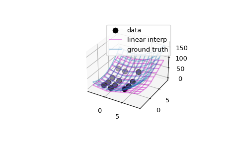
>>> import matplotlib.pyplot as plt
>>> fig = plt.figure()
>>> ax = fig.add_subplot(projection='3d')
>>> ax.scatter(xg.ravel(), yg.ravel(), data.ravel(),
...            s=60, c='k', label='data')

Evaluate and plot the interpolator on a finer grid

>>> xx = np.linspace(-4, 9, 31)
>>> yy = np.linspace(-4, 9, 31)
>>> X, Y = np.meshgrid(xx, yy, indexing='ij')

>>> # interpolator
>>> ax.plot_wireframe(X, Y, interp((X, Y)), rstride=3, cstride=3,
...                   alpha=0.4, color='m', label='linear interp')

>>> # ground truth
>>> ax.plot_wireframe(X, Y, ff(X, Y), rstride=3, cstride=3,
...                   alpha=0.4, label='ground truth')
>>> plt.legend()
>>> plt.show()

Other examples are given in the tutorial.

Go BackOpen In Tab