Multivariate data interpolation on a regular grid (RegularGridInterpolator)

Suppose you have N-dimensional data on a regular grid, and you want to interpolate it. In such a case, RegularGridInterpolator can be useful. Several interpolation strategies are supported: nearest-neighbor, linear, and tensor product splines of odd degree.

Strictly speaking, this class efficiently handles data given on rectilinear grids: hypercubic lattices with possibly unequal spacing between points. The number of points per dimension can be different for different dimensions.

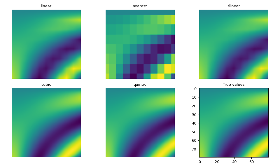
The following example demonstrates its use, and compares the interpolation results using each method.

>>> import numpy as np
>>> import matplotlib.pyplot as plt
>>> from scipy.interpolate import RegularGridInterpolator

Suppose we want to interpolate this 2-D function.

>>> def F(u, v):
...     return u * np.cos(u * v) + v * np.sin(u * v)

Suppose we only know some data on a regular grid.

>>> fit_points = [np.linspace(0, 3, 8), np.linspace(0, 3, 11)]
>>> values = F(*np.meshgrid(*fit_points, indexing='ij'))

Creating test points and true values for evaluations.

>>> ut, vt = np.meshgrid(np.linspace(0, 3, 80), np.linspace(0, 3, 80), indexing='ij')
>>> true_values = F(ut, vt)
>>> test_points = np.array([ut.ravel(), vt.ravel()]).T

We can create the interpolator and interpolate test points using each method.

>>> interp = RegularGridInterpolator(fit_points, values)
>>> fig, axes = plt.subplots(2, 3, figsize=(10, 6))
>>> axes = axes.ravel()
>>> fig_index = 0
>>> for method in ['linear', 'nearest', 'slinear', 'cubic', 'quintic']:
...     im = interp(test_points, method=method).reshape(80, 80)
...     axes[fig_index].imshow(im)
...     axes[fig_index].set_title(method)
...     axes[fig_index].axis("off")
...     fig_index += 1
>>> axes[fig_index].imshow(true_values)
>>> axes[fig_index].set_title("True values")
>>> fig.tight_layout()
>>> fig.show()

As expected, the higher degree spline interpolations are closest to the true values, though are more expensive to compute than with linear or nearest. The slinear interpolation also matches the linear interpolation.

If your data is such that spline methods produce ringing, you may consider using method="pchip", which uses the tensor product of PCHIP interpolators, a PchipInterpolator per dimension.

If you prefer a functional interface opposed to explicitly creating a class instance, the interpn convenience function offers the equivalent functionality.

Specifically, these two forms give identical results:

>>> from scipy.interpolate import interpn
>>> rgi = RegularGridInterpolator(fit_points, values)
>>> result_rgi = rgi(test_points)

and

>>> result_interpn = interpn(fit_points, values, test_points)
>>> np.allclose(result_rgi, result_interpn, atol=1e-15)
True

For data confined to an (N-1)-dimensional subspace of N-dimensional space, i.e. when one of the grid axes has length 1, the extrapolation along this axis is controlled by the fill_value keyword parameter:

>>> x = np.array([0, 5, 10])
>>> y = np.array([0])
>>> data = np.array([[0], [5], [10]])
>>> rgi = RegularGridInterpolator((x, y), data,
...                               bounds_error=False, fill_value=None)
>>> rgi([(2, 0), (2, 1), (2, -1)])   # extrapolates the value on the axis
array([2., 2., 2.])
>>> rgi.fill_value = -101
>>> rgi([(2, 0), (2, 1), (2, -1)])
array([2., -101., -101.])

Note

If the input data is such that input dimensions have incommensurate units and differ by many orders of magnitude, the interpolant may have numerical artifacts. Consider rescaling the data before interpolating.

Batch dimensions of values

Suppose you have a vector function \(f(x) = y\), where \(x\) and \(y\) are vectors, potentially of different lengths, and you want to sample the function on a grid of \(x\) values. One way to address this is to use the fact that RegularGridInterpolator allows values with trailing dimensions.

In accordance with how 1D interpolators interpret multidimensional arrays, the interpretation is that the first \(N\) dimensions of the values arrays are data dimensions (i.e. they correspond to the points defined by the grid argument), and the trailing dimensions are batch axes. Note that this disagrees with a usual NumPy broadcasting conventions, where broadcasting proceeds along the leading dimensions.

To illustrate:

>>> n = 5   # the number of batch components

>>> # make a 3D grid
>>> x1 = np.linspace(-np.pi, np.pi, 10)
>>> x2 = np.linspace(0.0, np.pi, 15)
>>> x3 = np.linspace(0.0, np.pi/2, 20)
>>> points = (x1, x2, x3)
>>>
>>> # define a function and sample it on the grid
>>> def f(x1, x2, x3, n):
...     lst = [np.sin(np.pi*x1/2) * np.exp(x2/2) + x3 + i for i in range(n)]
...     return np.asarray(lst)
>>>
>>> X1, X2, X3 = np.meshgrid(x1, x2, x3, indexing="ij")
>>> values = f(X1, X2, X3, n)
>>> values.shape
(5, 10, 15, 20)
>>>
>>> # prepare the data and construct the interpolator
>>> values = np.moveaxis(values, 0, -1)
>>> values.shape
(10, 15, 20, 5)     # the batch dimension is 5
>>> rgi = RegularGridInterpolator(points, values)
>>>
>>> # Coordinates to compute the interpolation at
>>> x = np.asarray([0.2, np.pi/2.1, np.pi/4.1])
>>>
# evaluate
>>> rgi(x).shape
(1, 5)

In this example, we evaluated a batch of \(n=5\) functions on a three-dimensional grid. In general, multiple batching dimensions are allowed, and the shape of the result follows by appending the batching shape (in this example, (5,)) to the shape of the input x (in this example, (1,)`).

Uniformly spaced data

If you are dealing with data on Cartesian grids with integer coordinates, e.g. resampling image data, these routines may not be the optimal choice. Consider using scipy.ndimage.map_coordinates instead.

For floating-point data on grids with equal spacing, map_coordinates can be easily wrapped into a RegularGridInterpolator look-alike. The following is a bare-bones example originating from the Johanness Buchner’s ‘regulargrid’ package:

class CartesianGridInterpolator:
    def __init__(self, points, values, method='linear'):
        self.limits = np.array([[min(x), max(x)] for x in points])
        self.values = np.asarray(values, dtype=float)
        self.order = {'linear': 1, 'cubic': 3, 'quintic': 5}[method]

    def __call__(self, xi):
        """
        `xi` here is an array-like (an array or a list) of points.

        Each "point" is an ndim-dimensional array_like, representing
        the coordinates of a point in ndim-dimensional space.
        """
        # transpose the xi array into the ``map_coordinates`` convention
        # which takes coordinates of a point along columns of a 2D array.
        xi = np.asarray(xi).T

        # convert from data coordinates to pixel coordinates
        ns = self.values.shape
        coords = [(n-1)*(val - lo) / (hi - lo)
                  for val, n, (lo, hi) in zip(xi, ns, self.limits)]

        # interpolate
        return map_coordinates(self.values, coords,
                               order=self.order,
                               cval=np.nan)  # fill_value

This wrapper can be used as a(n almost) drop-in replacement for the RegularGridInterpolator:

>>> x, y = np.arange(5), np.arange(6)
>>> xx, yy = np.meshgrid(x, y, indexing='ij')
>>> values = xx**3 + yy**3
>>> rgi = RegularGridInterpolator((x, y), values, method='linear')
>>> rgi([[1.5, 1.5], [3.5, 2.6]])
array([ 9. , 64.9])
>>> cgi = CartesianGridInterpolator((x, y), values, method='linear')
>>> cgi([[1.5, 1.5], [3.5, 2.6]])
array([ 9. , 64.9])

Note that the example above uses the map_coordinates boundary conditions. Thus, results of the cubic and quintic interpolations may differ from those of the RegularGridInterpolator. Refer to scipy.ndimage.map_coordinates documentation for more details on boundary conditions and other additional arguments. Finally, we note that this simplified example assumes that the input data is given in the ascending order.