Jarque-Bera goodness of fit test#
Suppose we wish to infer from measurements whether the weights of adult human
males in a medical study are not normally distributed [1]. The weights (lbs)
are recorded in the array x below.
import numpy as np
x = np.array([148, 154, 158, 160, 161, 162, 166, 170, 182, 195, 236])
The Jarque-Bera test scipy.stats.jarque_bera begins by computing a
statistic based on the sample skewness and kurtosis.
from scipy import stats
res = stats.jarque_bera(x)
res.statistic
np.float64(6.982848237344646)
Because the normal distribution has zero skewness and zero (“excess” or “Fisher”) kurtosis, the value of this statistic tends to be low for samples drawn from a normal distribution.
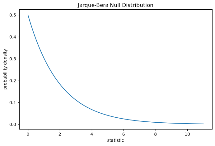
The test is performed by comparing the observed value of the statistic against the null distribution: the distribution of statistic values derived under the null hypothesis that the weights were drawn from a normal distribution.
For the Jarque-Bera test, the null distribution for very large samples is the
chi-squared distribution with two degrees of freedom.
import matplotlib.pyplot as plt

dist = stats.chi2(df=2)
jb_val = np.linspace(0, 11, 100)
pdf = dist.pdf(jb_val)
fig, ax = plt.subplots(figsize=(8, 5))

def jb_plot(ax):  # we'll reuse this
    ax.plot(jb_val, pdf)
    ax.set_title("Jarque-Bera Null Distribution")
    ax.set_xlabel("statistic")
    ax.set_ylabel("probability density")

jb_plot(ax)
plt.show();
The comparison is quantified by the p-value: the proportion of values in the null distribution greater than or equal to the observed value of the statistic.
fig, ax = plt.subplots(figsize=(8, 5))
jb_plot(ax)
pvalue = dist.sf(res.statistic)
annotation = (f'p-value={pvalue:.6f}\n(shaded area)')
props = dict(facecolor='black', width=1, headwidth=5, headlength=8)
_ = ax.annotate(annotation, (7.5, 0.01), (8, 0.05), arrowprops=props)
i = jb_val >= res.statistic  # indices of more extreme statistic values
ax.fill_between(jb_val[i], y1=0, y2=pdf[i])
ax.set_xlim(0, 11)
ax.set_ylim(0, 0.3)
plt.show()
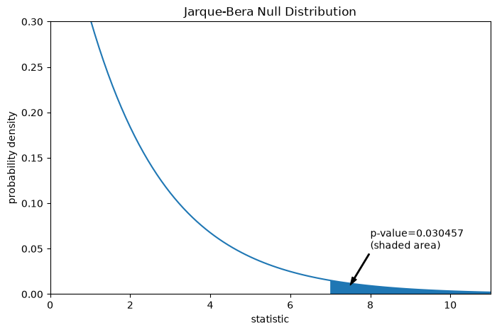
res.pvalue
np.float64(0.03045746622458189)
If the p-value is “small” - that is, if there is a low probability of sampling data from a normally distributed population that produces such an extreme value of the statistic - this may be taken as evidence against the null hypothesis in favor of the alternative: the weights were not drawn from a normal distribution. Note that:
The inverse is not true; that is, the test is not used to provide evidence for the null hypothesis.
The threshold for values that will be considered “small” is a choice that should be made before the data is analyzed [2] with consideration of the risks of both false positives (incorrectly rejecting the null hypothesis) and false negatives (failure to reject a false null hypothesis).
Note that the chi-squared distribution provides an asymptotic approximation
of the null distribution; it is only accurate for samples with many
observations. For small samples like ours, scipy.stats.monte_carlo_test
may provide a more accurate, albeit stochastic, approximation of the
exact p-value.
def statistic(x, axis):
    # underlying calculation of the Jarque Bera statistic
    s = stats.skew(x, axis=axis)
    k = stats.kurtosis(x, axis=axis)
    return x.shape[axis]/6 * (s**2 + k**2/4)

res = stats.monte_carlo_test(x, stats.norm.rvs, statistic,
                             alternative='greater')
fig, ax = plt.subplots(figsize=(8, 5))
jb_plot(ax)
ax.hist(res.null_distribution, np.linspace(0, 10, 50),
        density=True)
ax.legend(['asymptotic approximation (many observations)',
           'Monte Carlo approximation (11 observations)'])
plt.show()
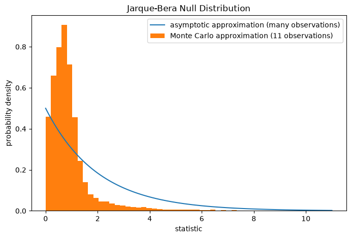
res.pvalue
np.float64(0.008)
Furthermore, despite their stochastic nature, p-values computed in this way can be used to exactly control the rate of false rejections of the null hypothesis [3].