monte_carlo_test#
- scipy.stats.monte_carlo_test(data, rvs, statistic, *, vectorized=None, n_resamples=9999, batch=None, alternative='two-sided', axis=0)[source]#
Perform a Monte Carlo hypothesis test.
data contains a sample or a sequence of one or more samples. rvs specifies the distribution(s) of the sample(s) in data under the null hypothesis. The value of statistic for the given data is compared against a Monte Carlo null distribution: the value of the statistic for each of n_resamples sets of samples generated using rvs. This gives the p-value, the probability of observing such an extreme value of the test statistic under the null hypothesis.
- Parameters:
- dataarray-like or sequence of array-like
An array or sequence of arrays of observations.
- rvscallable or tuple of callables
A callable or sequence of callables that generates random variates under the null hypothesis. Each element of rvs must be a callable that accepts keyword argument
size(e.g.rvs(size=(m, n))) and returns an N-d array sample of that shape. If rvs is a sequence, the number of callables in rvs must match the number of samples in data, i.e.len(rvs) == len(data). If rvs is a single callable, data is treated as a single sample.- statisticcallable
Statistic for which the p-value of the hypothesis test is to be calculated. statistic must be a callable that accepts a sample (e.g.
statistic(sample)) orlen(rvs)separate samples (e.g.statistic(samples1, sample2)if rvs contains two callables and data contains two samples) and returns the resulting statistic. If vectorized is setTrue, statistic must also accept a keyword argument axis and be vectorized to compute the statistic along the provided axis of the samples in data.- vectorizedbool, optional
If vectorized is set
False, statistic will not be passed keyword argument axis and is expected to calculate the statistic only for 1D samples. IfTrue, statistic will be passed keyword argument axis and is expected to calculate the statistic along axis when passed ND sample arrays. IfNone(default), vectorized will be setTrueifaxisis a parameter of statistic. Use of a vectorized statistic typically reduces computation time.- n_resamplesint, default: 9999
Number of samples drawn from each of the callables of rvs. Equivalently, the number statistic values under the null hypothesis used as the Monte Carlo null distribution.
- batchint, optional
The number of Monte Carlo samples to process in each call to statistic. Memory usage is O( batch *
sample.size[axis]). Default isNone, in which case batch equals n_resamples.- alternative{‘two-sided’, ‘less’, ‘greater’}
The alternative hypothesis for which the p-value is calculated. For each alternative, the p-value is defined as follows.
'greater': the percentage of the null distribution that is greater than or equal to the observed value of the test statistic.'less': the percentage of the null distribution that is less than or equal to the observed value of the test statistic.'two-sided': twice the smaller of the p-values above.
- axisint, default: 0
The axis of data (or each sample within data) over which to calculate the statistic.
- Returns:
- resMonteCarloTestResult
An object with attributes:
- statisticfloat or ndarray
The test statistic of the observed data.
- pvaluefloat or ndarray
The p-value for the given alternative.
- null_distributionndarray
The values of the test statistic generated under the null hypothesis.
Warning
The p-value is calculated by counting the elements of the null distribution that are as extreme or more extreme than the observed value of the statistic. Due to the use of finite precision arithmetic, some statistic functions return numerically distinct values when the theoretical values would be exactly equal. In some cases, this could lead to a large error in the calculated p-value.
monte_carlo_testguards against this by considering elements in the null distribution that are “close” (within a relative tolerance of 100 times the floating point epsilon of inexact dtypes) to the observed value of the test statistic as equal to the observed value of the test statistic. However, the user is advised to inspect the null distribution to assess whether this method of comparison is appropriate, and if not, calculate the p-value manually.
Notes
Array API Standard Support
monte_carlo_testhas experimental support for Python Array API Standard compatible backends in addition to NumPy. Please consider testing these features by setting an environment variableSCIPY_ARRAY_API=1and providing CuPy, PyTorch, JAX, or Dask arrays as array arguments. The following combinations of backend and device (or other capability) are supported.Library
CPU
GPU
NumPy
✅
n/a
CuPy
n/a
✅
PyTorch
✅
✅
JAX
✅
✅
Dask
✅
n/a
See Support for the array API standard for more information.
References
[1]B. Phipson and G. K. Smyth. “Permutation P-values Should Never Be Zero: Calculating Exact P-values When Permutations Are Randomly Drawn.” Statistical Applications in Genetics and Molecular Biology 9.1 (2010).
Examples
Suppose we wish to test whether a small sample has been drawn from a normal distribution. We decide that we will use the skew of the sample as a test statistic, and we will consider a p-value of 0.05 to be statistically significant.
>>> import numpy as np
>>> from scipy import stats
>>> def statistic(x, axis):
...     return stats.skew(x, axis)
After collecting our data, we calculate the observed value of the test statistic.
>>> rng = np.random.default_rng()
>>> x = stats.skewnorm.rvs(a=1, size=50, random_state=rng)
>>> statistic(x, axis=0)
0.12457412450240658
To determine the probability of observing such an extreme value of the skewness by chance if the sample were drawn from the normal distribution, we can perform a Monte Carlo hypothesis test. The test will draw many samples at random from their normal distribution, calculate the skewness of each sample, and compare our original skewness against this distribution to determine an approximate p-value.
>>> from scipy.stats import monte_carlo_test
>>> # because our statistic is vectorized, we pass `vectorized=True`
>>> rvs = lambda size: stats.norm.rvs(size=size, random_state=rng)
>>> res = monte_carlo_test(x, rvs, statistic, vectorized=True)
>>> print(res.statistic)
0.12457412450240658
>>> print(res.pvalue)
0.7012
The probability of obtaining a test statistic less than or equal to the observed value under the null hypothesis is ~70%. This is greater than our chosen threshold of 5%, so we cannot consider this to be significant evidence against the null hypothesis.
Note that this p-value essentially matches that of
scipy.stats.skewtest, which relies on an asymptotic distribution of a test statistic based on the sample skewness.>>> stats.skewtest(x).pvalue 0.6892046027110614
This asymptotic approximation is not valid for small sample sizes, but
monte_carlo_testcan be used with samples of any size.>>> x = stats.skewnorm.rvs(a=1, size=7, random_state=rng) >>> # stats.skewtest(x) would produce an error due to small sample >>> res = monte_carlo_test(x, rvs, statistic, vectorized=True)
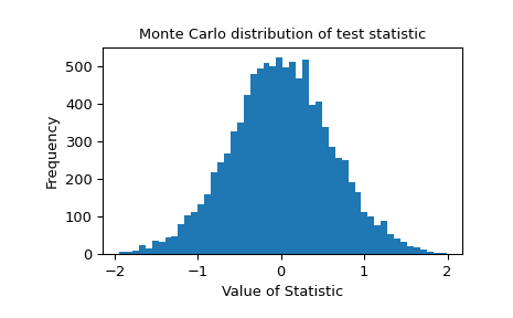
The Monte Carlo distribution of the test statistic is provided for further investigation.
>>> import matplotlib.pyplot as plt
>>> fig, ax = plt.subplots()
>>> ax.hist(res.null_distribution, bins=50)
>>> ax.set_title("Monte Carlo distribution of test statistic")
>>> ax.set_xlabel("Value of Statistic")
>>> ax.set_ylabel("Frequency")
>>> plt.show()