scipy.special.pseudo_huber#

scipy.special.pseudo_huber(delta, r, out=None) = <ufunc 'pseudo_huber'>#

Pseudo-Huber loss function.

p s e u d o_h u b e r (δ, r) = δ^{2} (\sqrt{1 + {(\frac{r}{δ})}^{2}} - 1)

$\mathrm{pseudo\_huber}(\delta, r) = \delta^2 \left( \sqrt{ 1 + \left( \frac{r}{\delta} \right)^2 } - 1 \right)$

Parameters:

deltaarray_like: Input array, indicating the soft quadratic vs. linear loss changepoint.
rarray_like: Input array, possibly representing residuals.
outndarray, optional: Optional output array for the function results

Returns:

resscalar or ndarray: The computed Pseudo-Huber loss function values.

See also

huber: Similar function which this function approximates

Notes

Like huber, pseudo_huber often serves as a robust loss function in statistics or machine learning to reduce the influence of outliers. Unlike huber, pseudo_huber is smooth.

Typically, r represents residuals, the difference between a model prediction and data. Then, for $|r|\leq\delta$ , pseudo_huber resembles the squared error and for $|r|>\delta$ the absolute error. This way, the Pseudo-Huber loss often achieves a fast convergence in model fitting for small residuals like the squared error loss function and still reduces the influence of outliers ( $|r|>\delta$ ) like the absolute error loss. As $\delta$ is the cutoff between squared and absolute error regimes, it has to be tuned carefully for each problem. pseudo_huber is also convex, making it suitable for gradient based optimization. [1] [2]

Added in version 0.15.0.

References

[1]

Hartley, Zisserman, “Multiple View Geometry in Computer Vision”. 2003. Cambridge University Press. p. 619

[2]

Charbonnier et al. “Deterministic edge-preserving regularization in computed imaging”. 1997. IEEE Trans. Image Processing. 6 (2): 298 - 311.

Examples

Import all necessary modules.

>>> import numpy as np
>>> from scipy.special import pseudo_huber, huber
>>> import matplotlib.pyplot as plt

Calculate the function for delta=1 at r=2.

>>> pseudo_huber(1., 2.)
1.2360679774997898

Calculate the function at r=2 for different delta by providing a list or NumPy array for delta.

>>> pseudo_huber([1., 2., 4.], 3.)
array([2.16227766, 3.21110255, 4.        ])

Calculate the function for delta=1 at several points by providing a list or NumPy array for r.

>>> pseudo_huber(2., np.array([1., 1.5, 3., 4.]))
array([0.47213595, 1.        , 3.21110255, 4.94427191])

The function can be calculated for different delta and r by providing arrays for both with compatible shapes for broadcasting.

>>> r = np.array([1., 2.5, 8., 10.])
>>> deltas = np.array([[1.], [5.], [9.]])
>>> print(r.shape, deltas.shape)
(4,) (3, 1)

>>> pseudo_huber(deltas, r)
array([[ 0.41421356,  1.6925824 ,  7.06225775,  9.04987562],
       [ 0.49509757,  2.95084972, 22.16990566, 30.90169944],
       [ 0.49846624,  3.06693762, 27.37435121, 40.08261642]])

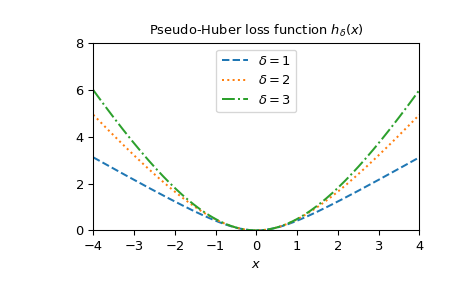
Plot the function for different delta.

>>> x = np.linspace(-4, 4, 500)
>>> deltas = [1, 2, 3]
>>> linestyles = ["dashed", "dotted", "dashdot"]
>>> fig, ax = plt.subplots()
>>> combined_plot_parameters = list(zip(deltas, linestyles))
>>> for delta, style in combined_plot_parameters:
...     ax.plot(x, pseudo_huber(delta, x), label=rf"$\delta={delta}$",
...             ls=style)
>>> ax.legend(loc="upper center")
>>> ax.set_xlabel("$x$")
>>> ax.set_title(r"Pseudo-Huber loss function $h_{\delta}(x)$")
>>> ax.set_xlim(-4, 4)
>>> ax.set_ylim(0, 8)
>>> plt.show()

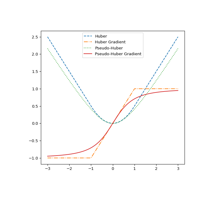
../../_images/scipy-special-pseudo_huber-1_00_00.png

Finally, illustrate the difference between huber and pseudo_huber by plotting them and their gradients with respect to r. The plot shows that pseudo_huber is continuously differentiable while huber is not at the points $\pm\delta$ .

>>> def huber_grad(delta, x):
...     grad = np.copy(x)
...     linear_area = np.argwhere(np.abs(x) > delta)
...     grad[linear_area]=delta*np.sign(x[linear_area])
...     return grad
>>> def pseudo_huber_grad(delta, x):
...     return x* (1+(x/delta)**2)**(-0.5)
>>> x=np.linspace(-3, 3, 500)
>>> delta = 1.
>>> fig, ax = plt.subplots(figsize=(7, 7))
>>> ax.plot(x, huber(delta, x), label="Huber", ls="dashed")
>>> ax.plot(x, huber_grad(delta, x), label="Huber Gradient", ls="dashdot")
>>> ax.plot(x, pseudo_huber(delta, x), label="Pseudo-Huber", ls="dotted")
>>> ax.plot(x, pseudo_huber_grad(delta, x), label="Pseudo-Huber Gradient",
...         ls="solid")
>>> ax.legend(loc="upper center")
>>> plt.show()

../../_images/scipy-special-pseudo_huber-1_01_00.png