scipy.special.huber#
- scipy.special.huber(delta, r, out=None) = <ufunc 'huber'>#
Huber loss function.
\[\begin{split}\text{huber}(\delta, r) = \begin{cases} \infty & \delta < 0 \\ \frac{1}{2}r^2 & 0 \le \delta, | r | \le \delta \\ \delta ( |r| - \frac{1}{2}\delta ) & \text{otherwise} \end{cases}\end{split}\]- Parameters:
- deltandarray
Input array, indicating the quadratic vs. linear loss changepoint.
- rndarray
Input array, possibly representing residuals.
- outndarray, optional
Optional output array for the function values
- Returns:
- scalar or ndarray
The computed Huber loss function values.
See also
pseudo_hubersmooth approximation of this function
Notes
huberis useful as a loss function in robust statistics or machine learning to reduce the influence of outliers as compared to the common squared error loss, residuals with a magnitude higher than delta are not squared [1].Typically, r represents residuals, the difference between a model prediction and data. Then, for \(|r|\leq\delta\),
huberresembles the squared error and for \(|r|>\delta\) the absolute error. This way, the Huber loss often achieves a fast convergence in model fitting for small residuals like the squared error loss function and still reduces the influence of outliers (\(|r|>\delta\)) like the absolute error loss. As \(\delta\) is the cutoff between squared and absolute error regimes, it has to be tuned carefully for each problem.huberis also convex, making it suitable for gradient based optimization.Added in version 0.15.0.
Array API Standard Support
huberhas experimental support for Python Array API Standard compatible backends in addition to NumPy. Please consider testing these features by setting an environment variableSCIPY_ARRAY_API=1and providing CuPy, PyTorch, JAX, or Dask arrays as array arguments. The following combinations of backend and device (or other capability) are supported.Library
CPU
GPU
NumPy
✅
n/a
CuPy
n/a
✅
PyTorch
✅
⛔
JAX
✅
⛔
Dask
✅
n/a
See Support for the array API standard for more information.
References
[1]Peter Huber. “Robust Estimation of a Location Parameter”, 1964. Annals of Statistics. 53 (1): 73 - 101.
Examples
Import all necessary modules.
>>> import numpy as np
>>> from scipy.special import huber
>>> import matplotlib.pyplot as plt
Compute the function for
delta=1atr=2>>> huber(1., 2.) 1.5
Compute the function for different delta by providing a NumPy array or list for delta.
>>> huber([1., 3., 5.], 4.)
array([3.5, 7.5, 8. ])
Compute the function at different points by providing a NumPy array or list for r.
>>> huber(2., np.array([1., 1.5, 3.]))
array([0.5  , 1.125, 4.   ])
The function can be calculated for different delta and r by providing arrays for both with compatible shapes for broadcasting.
>>> r = np.array([1., 2.5, 8., 10.])
>>> deltas = np.array([[1.], [5.], [9.]])
>>> print(r.shape, deltas.shape)
(4,) (3, 1)
>>> huber(deltas, r)
array([[ 0.5  ,  2.   ,  7.5  ,  9.5  ],
       [ 0.5  ,  3.125, 27.5  , 37.5  ],
       [ 0.5  ,  3.125, 32.   , 49.5  ]])
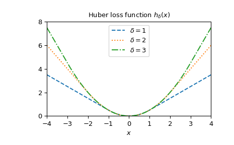
Plot the function for different delta.
>>> x = np.linspace(-4, 4, 500)
>>> deltas = [1, 2, 3]
>>> linestyles = ["dashed", "dotted", "dashdot"]
>>> fig, ax = plt.subplots()
>>> combined_plot_parameters = list(zip(deltas, linestyles))
>>> for delta, style in combined_plot_parameters:
...     ax.plot(x, huber(delta, x), label=fr"$\delta={delta}$", ls=style)
>>> ax.legend(loc="upper center")
>>> ax.set_xlabel("$x$")
>>> ax.set_title(r"Huber loss function $h_{\delta}(x)$")
>>> ax.set_xlim(-4, 4)
>>> ax.set_ylim(0, 8)
>>> plt.show()