scipy.special.dawsn#

scipy.special.dawsn(x, out=None) = <ufunc 'dawsn'>#

Dawson’s integral.

Computes

\[F(x) = e^{-x^2} \int_0^x e^{t^2} \, dt.\]

Parameters:

xarray_like: Real or complex-valued argument.
outndarray, optional: Optional output array for the function values.

Returns:

yscalar or ndarray: Value of the integral.

See also

wofz, erf, erfc, erfcx, erfi

Notes

Dawson’s integral is related to the imaginary error function by

\[F(x) = \frac{\sqrt{\pi}}{2} e^{-x^2} \operatorname{erfi}(x).\]

It satisfies the ordinary differential equation

\[F'(x) + 2xF(x) = 1, \qquad F(0) = 0.\]

For more details, see [1] and [2].

References

[1]

NIST Digital Library of Mathematical Functions, “Dawson’s Integral”. https://dlmf.nist.gov/7.2

[2]

Wikipedia, “Dawson function”. https://en.wikipedia.org/wiki/Dawson_function

[3]

Steven G. Johnson, Faddeeva W function implementation. http://ab-initio.mit.edu/Faddeeva

Examples

>>> import numpy as np
>>> from scipy.special import dawsn, erfi

Verify the relation between Dawson’s integral and erfi:

>>> x = np.linspace(-1, 1, 21)
>>> y = dawsn(x)
>>> y_erfi = np.sqrt(np.pi) * np.exp(-x**2) * erfi(x) / 2
>>> np.allclose(y, y_erfi)
True

The differential equation can also be checked numerically using a centered finite difference:

>>> eps = 1e-8
>>> dy = (dawsn(x + eps) - dawsn(x - eps)) / (2*eps)
>>> np.allclose(dy + 2*x*y, 1, rtol=0, atol=2e-8)
True

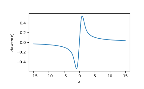
Plot the function over a wider interval:

>>> import matplotlib.pyplot as plt
>>> x = np.linspace(-15, 15, num=1000)
>>> plt.plot(x, dawsn(x))
>>> plt.xlabel('$x$')
>>> plt.ylabel('$F(x)$')
>>> plt.show()