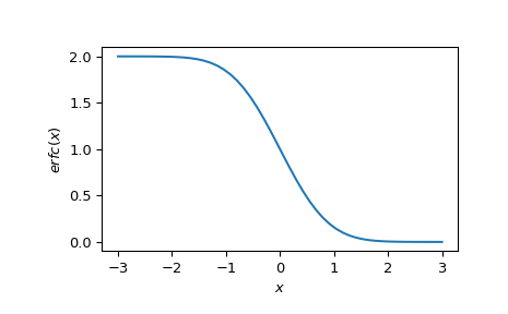
scipy.special.erfc#

scipy.special.erfc(x, out=None) = <ufunc 'erfc'>#

Complementary error function.

The complementary error function is defined as

\[\operatorname{erfc}(x) = 1 - \operatorname{erf}(x)\]

Parameters:

xarray_like: Real or complex valued argument
outndarray, optional: Optional output array for the function results

Returns:

scalar or ndarray: Values of the complementary error function

See also

erf, erfi, erfcx, dawsn, wofz

Notes

Array API Standard Support

erfc has support for Python Array API Standard compatible backends in addition to NumPy. The following combinations of backend and device (or other capability) are supported.

Library	CPU	GPU
NumPy	✅	n/a
CuPy	n/a	✅
PyTorch	✅	✅
JAX	✅	✅
Dask	✅	n/a

For the NumPy backend, this function supports all NumPy ufunc keyword arguments. Other backends may support out, but none of the other ufunc kwargs. out is typically supported for CuPy and PyTorch, but not currently in cases where SciPy relies on a generic Array API implementation or, for PyTorch on CPU, falls back to the NumPy backend. out is never supported for JAX because JAX arrays are immutable.

See Support for the array API standard for more information.

References

[1]

Steven G. Johnson, Faddeeva W function implementation. http://ab-initio.mit.edu/Faddeeva

Examples

In this example we consider modelling the instantaneous heating of a semi-infinite solid from its boundary at \(x=0\). This is governed by the heat equation

\[\frac{\partial T}{\partial t} = \frac{\partial^2 T}{\partial x^2}, \qquad x > 0, \quad t > 0,\]

with boundary conditions \(T(0,t) = 1\) and \(T(\infty,t) = 0\) and initial condition \(T(x,0) = 0\). Seeking a solution of the form \(T(x,t) = f(\eta)\) with \(\eta = x/\sqrt{t}\) transforms the problem into the following ordinary differential equation

\[f'' + \frac{\eta}{2} f' = 0, \qquad f(0) = 1, \quad f(\infty) = 0,\]

which has the solution \(f(\eta) = \operatorname{erfc}(\eta/2)\). We conclude the example by plotting the solution both as a function of \(\eta\) and as a function of \(x\) for different times.

>>> import numpy as np
>>> import matplotlib.pyplot as plt
>>> from scipy.special import erfc
>>> fig, (ax1, ax2) = plt.subplots(2, 1, layout="constrained", figsize=(5, 5))
>>> eta = np.linspace(0, 4)
>>> ax1.plot(eta, erfc(eta/2))
>>> ax1.set_xlabel(r'$\eta$')
>>> ax1.set_ylabel(r'$f(\eta)$')
>>> x = np.linspace(0, 2, num=100)
>>> for t in [0.001, 0.01, 0.1, 0.5, 1]:
...     ax2.plot(x, erfc(x/(2*np.sqrt(t))), label=f't={t}')
>>> ax2.set_xlabel(r'$x$')
>>> ax2.set_ylabel(r'$T(x,t)$')
>>> ax2.legend()
>>> plt.show()