scipy.signal.windows.

lanczos

scipy.signal.windows.lanczos(M, *, sym=True, xp=None, device=None)

Return a Lanczos window also known as a sinc window.

Parameters:

Mint

Number of points in the output window. If zero, an empty array is returned. An exception is thrown when it is negative.

symbool, optional

When True (default), generates a symmetric window, for use in filter design. When False, generates a periodic window, for use in spectral analysis.

xparray_namespace, optional

Optional array namespace. Should be compatible with the array API standard, or supported by array-api-compat. Default: numpy

device: any

optional device specification for output. Should match one of the supported device specification in xp.

Returns:

wndarray

The window, with the maximum value normalized to 1 (though the value 1 does not appear if M is even and sym is True).

Notes

The Lanczos window is defined as

\[w(n) = sinc \left( \frac{2n}{M - 1} - 1 \right)\]

where

\[sinc(x) = \frac{\sin(\pi x)}{\pi x}\]

The Lanczos window has reduced Gibbs oscillations and is widely used for filtering climate timeseries with good properties in the physical and spectral domains.

Added in version 1.10.

Array API Standard Support

lanczos has experimental support for Python Array API Standard compatible backends in addition to NumPy. Please consider testing these features by setting an environment variable SCIPY_ARRAY_API=1 and providing CuPy, PyTorch, JAX, or Dask arrays as array arguments. The following combinations of backend and device (or other capability) are supported.

Library	CPU	GPU
NumPy	✅	n/a
CuPy	n/a	✅
PyTorch	✅	✅
JAX	✅	✅
Dask	✅	n/a

See Support for the array API standard for more information.

References

[1]

Lanczos, C., and Teichmann, T. (1957). Applied analysis. Physics Today, 10, 44.

[2]

Duchon C. E. (1979) Lanczos Filtering in One and Two Dimensions. Journal of Applied Meteorology, Vol 18, pp 1016-1022.

[3]

Thomson, R. E. and Emery, W. J. (2014) Data Analysis Methods in Physical Oceanography (Third Edition), Elsevier, pp 593-637.

[4]

Wikipedia, “Window function”, http://en.wikipedia.org/wiki/Window_function

Examples

Try it in your browser!

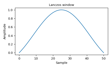
Plot the window

>>> import numpy as np
>>> from scipy.signal.windows import lanczos
>>> from scipy.fft import fft, fftshift
>>> import matplotlib.pyplot as plt
>>> fig, ax = plt.subplots(1)
>>> window = lanczos(51)
>>> ax.plot(window)
>>> ax.set_title("Lanczos window")
>>> ax.set_ylabel("Amplitude")
>>> ax.set_xlabel("Sample")
>>> fig.tight_layout()
>>> plt.show()

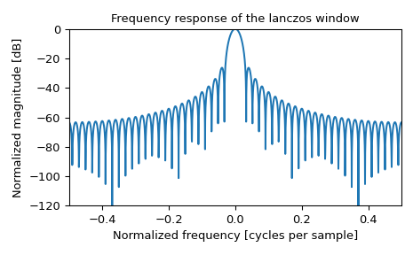
and its frequency response:

>>> fig, ax = plt.subplots(1)
>>> A = fft(window, 2048) / (len(window)/2.0)
>>> freq = np.linspace(-0.5, 0.5, len(A))
>>> response = 20 * np.log10(np.abs(fftshift(A / abs(A).max())))
>>> ax.plot(freq, response)
>>> ax.set_xlim(-0.5, 0.5)
>>> ax.set_ylim(-120, 0)
>>> ax.set_title("Frequency response of the lanczos window")
>>> ax.set_ylabel("Normalized magnitude [dB]")
>>> ax.set_xlabel("Normalized frequency [cycles per sample]")
>>> fig.tight_layout()
>>> plt.show()

Go BackOpen In Tab