scipy.signal.windows.

chebwin

scipy.signal.windows.chebwin(M, at, sym=True)

Return a Dolph-Chebyshev window.

Parameters:

Mint

Number of points in the output window. If zero, an empty array is returned. An exception is thrown when it is negative.

atfloat

Attenuation (in dB).

symbool, optional

When True (default), generates a symmetric window, for use in filter design. When False, generates a periodic window, for use in spectral analysis.

Returns:

wndarray

The window, with the maximum value always normalized to 1

Notes

This window optimizes for the narrowest main lobe width for a given order M and sidelobe equiripple attenuation at, using Chebyshev polynomials. It was originally developed by Dolph to optimize the directionality of radio antenna arrays.

Unlike most windows, the Dolph-Chebyshev is defined in terms of its frequency response:

\[W(k) = \frac {\cos\{M \cos^{-1}[\beta \cos(\frac{\pi k}{M})]\}} {\cosh[M \cosh^{-1}(\beta)]}\]

where

\[\beta = \cosh \left [\frac{1}{M} \cosh^{-1}(10^\frac{A}{20}) \right ]\]

and 0 <= abs(k) <= M-1. A is the attenuation in decibels (at).

The time domain window is then generated using the IFFT, so power-of-two M are the fastest to generate, and prime number M are the slowest.

The equiripple condition in the frequency domain creates impulses in the time domain, which appear at the ends of the window.

References

[1]

C. Dolph, “A current distribution for broadside arrays which optimizes the relationship between beam width and side-lobe level”, Proceedings of the IEEE, Vol. 34, Issue 6

[2]

Peter Lynch, “The Dolph-Chebyshev Window: A Simple Optimal Filter”, American Meteorological Society (April 1997) http://mathsci.ucd.ie/~plynch/Publications/Dolph.pdf

[3]

F. J. Harris, “On the use of windows for harmonic analysis with the discrete Fourier transforms”, Proceedings of the IEEE, Vol. 66, No. 1, January 1978

Examples

Try it in your browser!

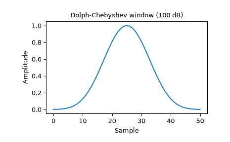
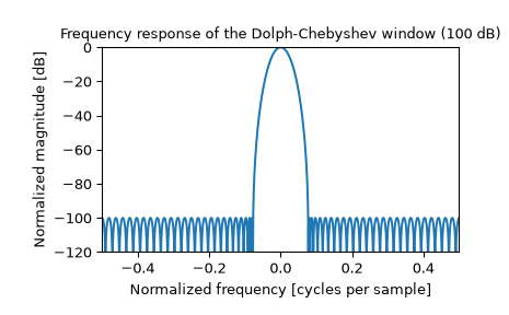
Plot the window and its frequency response:

>>> import numpy as np
>>> from scipy import signal
>>> from scipy.fft import fft, fftshift
>>> import matplotlib.pyplot as plt

>>> window = signal.windows.chebwin(51, at=100)
>>> plt.plot(window)
>>> plt.title("Dolph-Chebyshev window (100 dB)")
>>> plt.ylabel("Amplitude")
>>> plt.xlabel("Sample")

>>> plt.figure()
>>> A = fft(window, 2048) / (len(window)/2.0)
>>> freq = np.linspace(-0.5, 0.5, len(A))
>>> response = 20 * np.log10(np.abs(fftshift(A / abs(A).max())))
>>> plt.plot(freq, response)
>>> plt.axis([-0.5, 0.5, -120, 0])
>>> plt.title("Frequency response of the Dolph-Chebyshev window (100 dB)")
>>> plt.ylabel("Normalized magnitude [dB]")
>>> plt.xlabel("Normalized frequency [cycles per sample]")

Go BackOpen In Tab