scipy.signal.windows.

boxcar

scipy.signal.windows.boxcar(M, sym=True, *, xp=None, device=None)

Return a boxcar or rectangular window.

Also known as a rectangular window or Dirichlet window. This is equivalent to no window at all.

Parameters:

Mint

Number of points in the output window. If zero, an empty array is returned. An exception is thrown when it is negative.

symbool, optional

Whether the window is symmetric. (Has no effect for boxcar.)

xparray_namespace, optional

Optional array namespace. Should be compatible with the array API standard, or supported by array-api-compat. Default: numpy

deviceany

optional device specification for output. Should match one of the supported device specification in xp.

Returns:

wndarray

The window, i.e., w = np.ones(M).

Notes

Note that this function differs from the continuous-time “rect” function [1] by not returning 1/2 at its borders.

The Fourier transform of a continuous-time boxcar window can be expressed as

\[W(f) = \tau\operatorname{sinc}(\tau f) = \frac{\sin(\pi\tau f)}{\pi f} \,,\]

with \(\tau = M T\) being the window width and \(T\) the sampling interval. Eq. (4) in the The Discrete Fourier Transform section of the SciPy User Guide can be used to determine the values of the discrete Fourier transform (aka FFT), i.e.,

\[W[l] := \frac{1}{T\gamma} W(l\Delta f) = \frac{M}{\gamma}\operatorname{sinc}(l) \,, \qquad \Delta f := 1 / \tau = 1/ (MT) \,.\]

Here, \(\gamma\) is the FFT normalization constant (default: \(\gamma=1\)). \(W[l]\) is zero for nonzero integer values of \(l\) and its sidelobes decrease on the order of \(O(|l|^{-1})\).

For many applications, like calculating a magnitude spectrum in the example below, a normalized window is needed. Consult the Spectral Analysis section of the SciPy User Guide for details.

Array API Standard Support

boxcar has experimental support for Python Array API Standard compatible backends in addition to NumPy. Please consider testing these features by setting an environment variable SCIPY_ARRAY_API=1 and providing CuPy, PyTorch, JAX, or Dask arrays as array arguments. The following combinations of backend and device (or other capability) are supported.

Library	CPU	GPU
NumPy	✅	n/a
CuPy	n/a	✅
PyTorch	✅	✅
JAX	✅	✅
Dask	✅	n/a

See Support for the array API standard for more information.

References

[1]

“Rectangular function”, Wikipedia, https://en.wikipedia.org/wiki/Rectangular_function

Examples

Try it in your browser!

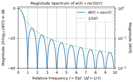
The following example compares a 10-sample boxcar window to its corresponding rect function. The upper plot depicts the amplitudes, whereas the corresponding magnitude spectra are shown in the lower plot. A standard resolution spectrum and a high resolution one, which is zero-padded by factor 16, are shown of the boxcar window. That the boxcar spectrum does not coincide everywhere with the rect function spectrum is due to the underlying continuous-time function of the boxcar window being a 10-term Fourier series approximation of the rect function.

>>> import numpy as np
>>> from matplotlib import pyplot as plt
>>> from scipy.fft import fft, fftfreq, fftshift
>>> from scipy.signal.windows import boxcar
...
>>> N, T = 10, 1/10  # number of samples and sampling interval in seconds
>>> t_w = np.arange(N) * T  # sample times
>>> w = boxcar(N)  # boxcar window
...
>>> W = fft(w) / sum(w)  # amplitude spectrum of w
>>> f_W = fftfreq(N, T)  # frequencies of W in Hz
>>> W16 = fftshift(fft(w, n=16*N)) / sum(w)  # zero-padded amplitude spectrum
>>> f_W16 = fftshift(fftfreq(N*16, T))  # frequencies of W16 in Hz
...
>>> # rect function in the Fourier domain:
>>> f_R = np.linspace(-((N + 2) // 2), (N + 1) // 2, 100, endpoint=True)
>>> R = np.sinc(f_R)
...
>>> _, (ax0, ax1) = plt.subplots(2, 1, figsize=(5, 4.5), constrained_layout=True)
>>> ax0.set_title(r"Boxcar window with corresponding rect function")
>>> ax0.set(ylabel="Amplitude", xlim=(-0.5, 1.5),
...         xlabel=rf"Time $t$ in seconds (${N}$ samples with interval ${T=}\,$s)")
>>> ax0.plot([[-.5,  0,  1], [ 0,  1, 1.5]], [[0, 1, 0], [0, 1, 0]], 'C0-',
...          alpha=0.5, label=(r"$w_r(t) = $rect$(t-\frac{1}{2})$", None, None))
>>> ax0.plot([[0, 1]], [[0.5, 0.5]], 'C0.-', alpha=0.5)  # mark border values of 1/2
>>> ax0.plot(t_w, w, 'C1o', label="Boxcar window")
>>> ax1.set_title(r"Magnitude Spectrum")
>>> ax1.set(ylabel="Magnitude", xlim=(f_R[0], f_R[-1]),
...         xlabel=rf"Frequency $f$ in hertz ($\Delta f = {f_W[1]:g}\,$Hz)")
>>> ax1.plot(f_R, abs(R), 'C0-', alpha=0.5, label="$W_r(f) = $sinc$(f)$")
>>> ax1.plot(f_W, abs(W), 'C1o', label=r"$W_r[l] = $sinc$(l\Delta f)$")
>>> ax1.plot(f_W16, abs(W16), 'C1--', alpha=0.5, label="zero-padded $W_r[l]$")
>>> for ax_, l_ in zip((ax0, ax1), ('lower center', 'best')):
...     ax_.legend(loc=l_)
...     ax_.grid(True)
>>> plt.show()

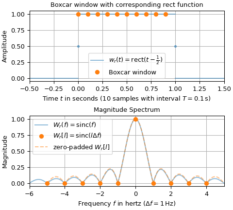
The following plot shows a logarithmically scaled version of the magnitude spectrum. The x-axis has been rescaled to correspond to the FFT-bin number. The dashed green line represents the approximate sidelobe height.

>>> import numpy as np
>>> from matplotlib import pyplot as plt
...
>>> f = np.arange(0, 10, 0.01)
>>> W_abs = abs(np.sinc(f))
>>> W_dB = np.where(W_abs > 0, 20*np.log10(W_abs), -1e250)
...
>>> f_Y = np.linspace(.5, f[-1], 100)
>>> Y_dB = 20*np.log10(1 / (np.pi*f_Y))
...
>>> _, ax0 = plt.subplots(constrained_layout=True)
>>> ax0.set_title(r"Magnitude Spectrum of $w(t) = $rect$(t/\tau)$")
>>> ax0.set(ylabel=r"Magnitude $20\,\log_{10} |W(l)|$ in dB", ylim=(-40, 1),
...         xlabel=r"Relative Frequency $l=f/\Delta f\ $ ($\Delta f = 1/\tau$)",
...         xlim=(f[0], f[-1]), yticks=[-40, -20, 0], xticks=np.arange(11))
>>> ax0.plot(f, W_dB, label="$W(l) = $sinc$(l)$")
>>> ax0.plot(f_Y, Y_dB, 'C2--', alpha=0.5, label=r"$1 / (\pi l)$")
>>> ax0.legend()
>>> ax0.grid(True)
>>> ax1 = ax0.twinx() # create right y-axis with logarithmic scaling:
>>> ax1.set_ylabel("Magnitude $|W(f)|$", rotation=-90, labelpad=15)
>>> ax1.set(ylim=(1e-2, 10**(1/20)), yscale="log")
>>> plt.show()

Go BackOpen In Tab