scipy.signal.

ellip

scipy.signal.ellip(N, rp, rs, Wn, btype='low', analog=False, output='ba', fs=None)

Elliptic (Cauer) digital and analog filter design.

Design an Nth-order digital or analog elliptic filter and return the filter coefficients.

Parameters:

Nint

The order of the filter.

rpfloat

The maximum ripple allowed below unity gain in the passband. Specified in decibels, as a positive number.

rsfloat

The minimum attenuation required in the stop band. Specified in decibels, as a positive number.

Wnarray_like

A scalar or length-2 sequence giving the critical frequencies. For elliptic filters, this is the point in the transition band at which the gain first drops below -rp.

For digital filters, Wn are in the same units as fs. By default, fs is 2 half-cycles/sample, so these are normalized from 0 to 1, where 1 is the Nyquist frequency. (Wn is thus in half-cycles / sample.)

For analog filters, Wn is an angular frequency (e.g., rad/s).

btype{‘lowpass’, ‘highpass’, ‘bandpass’, ‘bandstop’}, optional

The type of filter. Default is ‘lowpass’.

analogbool, optional

When True, return an analog filter, otherwise a digital filter is returned.

output{‘ba’, ‘zpk’, ‘sos’}, optional

Type of output: numerator/denominator (‘ba’), pole-zero (‘zpk’), or second-order sections (‘sos’). Default is ‘ba’ for backwards compatibility, but ‘sos’ should be used for general-purpose filtering.

fsfloat, optional

The sampling frequency of the digital system.

Added in version 1.2.0.

Returns:

b, andarray, ndarray

Numerator (b) and denominator (a) polynomials of the IIR filter. Only returned if output='ba'.

z, p, kndarray, ndarray, float

Zeros, poles, and system gain of the IIR filter transfer function. Only returned if output='zpk'.

sosndarray

Second-order sections representation of the IIR filter. Only returned if output='sos'.

See also

ellipord, ellipap

Notes

Also known as Cauer or Zolotarev filters, the elliptical filter maximizes the rate of transition between the frequency response’s passband and stopband, at the expense of ripple in both, and increased ringing in the step response.

As rp approaches 0, the elliptical filter becomes a Chebyshev type II filter (cheby2). As rs approaches 0, it becomes a Chebyshev type I filter (cheby1). As both approach 0, it becomes a Butterworth filter (butter).

The equiripple passband has N maxima or minima (for example, a 5th-order filter has 3 maxima and 2 minima). Consequently, the DC gain is unity for odd-order filters, or -rp dB for even-order filters.

The 'sos' output parameter was added in 0.16.0.

The current behavior is for ndarray outputs to have 64 bit precision (float64 or complex128) regardless of the dtype of Wn but outputs may respect the dtype of Wn in a future version.

Array API Standard Support

ellip has experimental support for Python Array API Standard compatible backends in addition to NumPy. Please consider testing these features by setting an environment variable SCIPY_ARRAY_API=1 and providing CuPy, PyTorch, JAX, or Dask arrays as array arguments. The following combinations of backend and device (or other capability) are supported.

Library	CPU	GPU
NumPy	✅	n/a
CuPy	n/a	✅
PyTorch	✅	⛔
JAX	⚠️ no JIT	⛔
Dask	⚠️ computes graph	n/a

See Support for the array API standard for more information.

Examples

Try it in your browser!

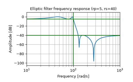
Design an analog filter and plot its frequency response, showing the critical points:

>>> from scipy import signal
>>> import matplotlib.pyplot as plt
>>> import numpy as np

>>> b, a = signal.ellip(4, 5, 40, 100, 'low', analog=True)
>>> w, h = signal.freqs(b, a)
>>> plt.semilogx(w, 20 * np.log10(abs(h)))
>>> plt.title('Elliptic filter frequency response (rp=5, rs=40)')
>>> plt.xlabel('Frequency [rad/s]')
>>> plt.ylabel('Amplitude [dB]')
>>> plt.margins(0, 0.1)
>>> plt.grid(which='both', axis='both')
>>> plt.axvline(100, color='green') # cutoff frequency
>>> plt.axhline(-40, color='green') # rs
>>> plt.axhline(-5, color='green') # rp
>>> plt.show()

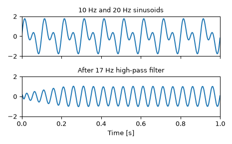
Generate a signal made up of 10 Hz and 20 Hz, sampled at 1 kHz

>>> t = np.linspace(0, 1, 1000, False)  # 1 second
>>> sig = np.sin(2*np.pi*10*t) + np.sin(2*np.pi*20*t)
>>> fig, (ax1, ax2) = plt.subplots(2, 1, sharex=True)
>>> ax1.plot(t, sig)
>>> ax1.set_title('10 Hz and 20 Hz sinusoids')
>>> ax1.axis([0, 1, -2, 2])

Design a digital high-pass filter at 17 Hz to remove the 10 Hz tone, and apply it to the signal. (It’s recommended to use second-order sections format when filtering, to avoid numerical error with transfer function (ba) format):

>>> sos = signal.ellip(8, 1, 100, 17, 'hp', fs=1000, output='sos')
>>> filtered = signal.sosfilt(sos, sig)
>>> ax2.plot(t, filtered)
>>> ax2.set_title('After 17 Hz high-pass filter')
>>> ax2.axis([0, 1, -2, 2])
>>> ax2.set_xlabel('Time [s]')
>>> plt.tight_layout()
>>> plt.show()

Go BackOpen In Tab