scipy.signal.

butter

scipy.signal.butter(N, Wn, btype='low', analog=False, output='ba', fs=None)

Butterworth digital and analog filter design.

Design an Nth-order digital or analog Butterworth filter and return the filter coefficients.

Parameters:

Nint

The order of the filter. For ‘bandpass’ and ‘bandstop’ filters, the resulting order of the final second-order sections (‘sos’) matrix is 2*N, with N the number of biquad sections of the desired system.

Wnarray_like

The critical frequency or frequencies. For lowpass and highpass filters, Wn is a scalar; for bandpass and bandstop filters, Wn is a length-2 sequence.

For a Butterworth filter, this is the point at which the gain drops to 1/sqrt(2) that of the passband (the “-3 dB point”).

For digital filters, if fs is not specified, Wn units are normalized from 0 to 1, where 1 is the Nyquist frequency (Wn is thus in half cycles / sample and defined as 2*critical frequencies / fs). If fs is specified, Wn is in the same units as fs.

For analog filters, Wn is an angular frequency (e.g. rad/s).

btype{‘lowpass’, ‘highpass’, ‘bandpass’, ‘bandstop’}, optional

The type of filter. Default is ‘lowpass’.

analogbool, optional

When True, return an analog filter, otherwise a digital filter is returned.

output{‘ba’, ‘zpk’, ‘sos’}, optional

Type of output: numerator/denominator (‘ba’), pole-zero (‘zpk’), or second-order sections (‘sos’). Default is ‘ba’ for backwards compatibility, but ‘sos’ should be used for general-purpose filtering.

fsfloat, optional

The sampling frequency of the digital system.

Added in version 1.2.0.

Returns:

b, andarray, ndarray

Numerator (b) and denominator (a) polynomials of the IIR filter. Only returned if output='ba'.

z, p, kndarray, ndarray, float

Zeros, poles, and system gain of the IIR filter transfer function. Only returned if output='zpk'.

sosndarray

Second-order sections representation of the IIR filter. Only returned if output='sos'.

See also

buttord, buttap

Notes

The Butterworth filter has maximally flat frequency response in the passband.

The 'sos' output parameter was added in 0.16.0.

If the transfer function form [b, a] is requested, numerical problems can occur since the conversion between roots and the polynomial coefficients is a numerically sensitive operation, even for N >= 4. It is recommended to work with the SOS representation.

Warning

Designing high-order and narrowband IIR filters in TF form can result in unstable or incorrect filtering due to floating point numerical precision issues. Consider inspecting output filter characteristics freqz or designing the filters with second-order sections via output='sos'.

The current behavior is for ndarray outputs to have 64 bit precision (float64 or complex128) regardless of the dtype of Wn but outputs may respect the dtype of Wn in a future version.

Array API Standard Support

butter has experimental support for Python Array API Standard compatible backends in addition to NumPy. Please consider testing these features by setting an environment variable SCIPY_ARRAY_API=1 and providing CuPy, PyTorch, JAX, or Dask arrays as array arguments. The following combinations of backend and device (or other capability) are supported.

Library	CPU	GPU
NumPy	✅	n/a
CuPy	n/a	✅
PyTorch	✅	⛔
JAX	⚠️ no JIT	⛔
Dask	⚠️ computes graph	n/a

See Support for the array API standard for more information.

Examples

Try it in your browser!

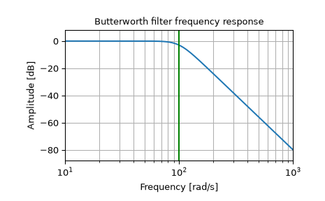
Design an analog filter and plot its frequency response, showing the critical points:

>>> from scipy import signal
>>> import matplotlib.pyplot as plt
>>> import numpy as np

>>> b, a = signal.butter(4, 100, 'low', analog=True)
>>> w, h = signal.freqs(b, a)
>>> plt.semilogx(w, 20 * np.log10(abs(h)))
>>> plt.title('Butterworth filter frequency response')
>>> plt.xlabel('Frequency [rad/s]')
>>> plt.ylabel('Amplitude [dB]')
>>> plt.margins(0, 0.1)
>>> plt.grid(which='both', axis='both')
>>> plt.axvline(100, color='green') # cutoff frequency
>>> plt.show()

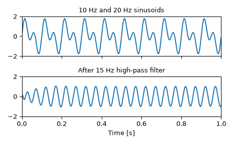
Generate a signal made up of 10 Hz and 20 Hz, sampled at 1 kHz

>>> t = np.linspace(0, 1, 1000, False)  # 1 second
>>> sig = np.sin(2*np.pi*10*t) + np.sin(2*np.pi*20*t)
>>> fig, (ax1, ax2) = plt.subplots(2, 1, sharex=True)
>>> ax1.plot(t, sig)
>>> ax1.set_title('10 Hz and 20 Hz sinusoids')
>>> ax1.axis([0, 1, -2, 2])

Design a digital high-pass filter at 15 Hz to remove the 10 Hz tone, and apply it to the signal. (It’s recommended to use second-order sections format when filtering, to avoid numerical error with transfer function (ba) format):

>>> sos = signal.butter(10, 15, 'hp', fs=1000, output='sos')
>>> filtered = signal.sosfilt(sos, sig)
>>> ax2.plot(t, filtered)
>>> ax2.set_title('After 15 Hz high-pass filter')
>>> ax2.axis([0, 1, -2, 2])
>>> ax2.set_xlabel('Time [s]')
>>> plt.tight_layout()
>>> plt.show()

Go BackOpen In Tab