scipy.signal.

cspline1d#

scipy.signal.cspline1d(signal, lamb=0.0)[source]#

Compute cubic spline coefficients for rank-1 array.

Find the cubic spline coefficients for a 1-D signal assuming mirror-symmetric boundary conditions. To obtain the signal back from the spline representation mirror-symmetric-convolve these coefficients with a length 3 FIR window [1.0, 4.0, 1.0]/ 6.0 .

Parameters:

signalndarray: A rank-1 array representing samples of a signal.
lambfloat, optional: Smoothing coefficient, default is 0.0.

Returns:

cndarray: Cubic spline coefficients.

See also

cspline1d_eval: Evaluate a cubic spline at the new set of points.

Notes

Array API Standard Support

cspline1d has experimental support for Python Array API Standard compatible backends in addition to NumPy. Please consider testing these features by setting an environment variable SCIPY_ARRAY_API=1 and providing CuPy, PyTorch, JAX, or Dask arrays as array arguments. The following combinations of backend and device (or other capability) are supported.

Library	CPU	GPU
NumPy	✅	n/a
CuPy	n/a	✅
PyTorch	✅	⛔
JAX	⚠️ no JIT	⛔
Dask	⚠️ computes graph	n/a

See Support for the array API standard for more information.

Examples

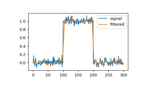
We can filter a signal to reduce and smooth out high-frequency noise with a cubic spline:

>>> import numpy as np
>>> import matplotlib.pyplot as plt
>>> from scipy.signal import cspline1d, cspline1d_eval
>>> rng = np.random.default_rng()
>>> sig = np.repeat([0., 1., 0.], 100)
>>> sig += rng.standard_normal(len(sig))*0.05  # add noise
>>> time = np.linspace(0, len(sig))
>>> filtered = cspline1d_eval(cspline1d(sig), time)
>>> plt.plot(sig, label="signal")
>>> plt.plot(time, filtered, label="filtered")
>>> plt.legend()
>>> plt.show()

../../_images/scipy-signal-cspline1d-1.png