scipy.signal.

qspline1d#

scipy.signal.qspline1d(signal, lamb=0.0)[source]#

Compute quadratic spline coefficients for rank-1 array.

Parameters:

signalndarray: A rank-1 array representing samples of a signal.
lambfloat, optional: Smoothing coefficient (must be zero for now).

Returns:

cndarray: Quadratic spline coefficients.

See also

qspline1d_eval: Evaluate a quadratic spline at the new set of points.

Notes

Find the quadratic spline coefficients for a 1-D signal assuming mirror-symmetric boundary conditions. To obtain the signal back from the spline representation mirror-symmetric-convolve these coefficients with a length 3 FIR window [1.0, 6.0, 1.0]/ 8.0 .

Array API Standard Support

qspline1d has experimental support for Python Array API Standard compatible backends in addition to NumPy. Please consider testing these features by setting an environment variable SCIPY_ARRAY_API=1 and providing CuPy, PyTorch, JAX, or Dask arrays as array arguments. The following combinations of backend and device (or other capability) are supported.

Library	CPU	GPU
NumPy	✅	n/a
CuPy	n/a	✅
PyTorch	✅	⛔
JAX	⚠️ no JIT	⛔
Dask	⚠️ computes graph	n/a

See Support for the array API standard for more information.

Examples

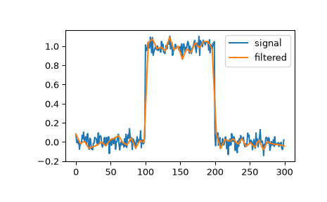
We can filter a signal to reduce and smooth out high-frequency noise with a quadratic spline:

>>> import numpy as np
>>> import matplotlib.pyplot as plt
>>> from scipy.signal import qspline1d, qspline1d_eval
>>> rng = np.random.default_rng()
>>> sig = np.repeat([0., 1., 0.], 100)
>>> sig += rng.standard_normal(len(sig))*0.05  # add noise
>>> time = np.linspace(0, len(sig))
>>> filtered = qspline1d_eval(qspline1d(sig), time)
>>> plt.plot(sig, label="signal")
>>> plt.plot(time, filtered, label="filtered")
>>> plt.legend()
>>> plt.show()

../../_images/scipy-signal-qspline1d-1.png