scipy.signal.

cspline1d_eval

scipy.signal.cspline1d_eval(cj, newx, dx=1.0, x0=0)

Evaluate a cubic spline at the new set of points.

dx is the old sample-spacing while x0 was the old origin. In other-words the old-sample points (knot-points) for which the cj represent spline coefficients were at equally-spaced points of:

oldx = x0 + j*dx j=0…N-1, with N=len(cj)

Edges are handled using mirror-symmetric boundary conditions.

Parameters:

cjndarray

cublic spline coefficients

newxndarray

New set of points.

dxfloat, optional

Old sample-spacing, the default value is 1.0.

x0int, optional

Old origin, the default value is 0.

Returns:

resndarray

Evaluated a cubic spline points.

See also

cspline1d

Compute cubic spline coefficients for rank-1 array.

Examples

Try it in your browser!

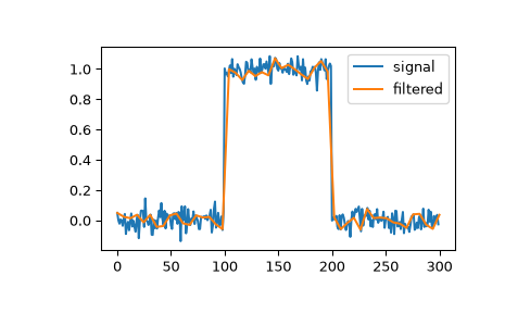
We can filter a signal to reduce and smooth out high-frequency noise with a cubic spline:

>>> import numpy as np
>>> import matplotlib.pyplot as plt
>>> from scipy.signal import cspline1d, cspline1d_eval
>>> rng = np.random.default_rng()
>>> sig = np.repeat([0., 1., 0.], 100)
>>> sig += rng.standard_normal(len(sig))*0.05  # add noise
>>> time = np.linspace(0, len(sig))
>>> filtered = cspline1d_eval(cspline1d(sig), time)
>>> plt.plot(sig, label="signal")
>>> plt.plot(time, filtered, label="filtered")
>>> plt.legend()
>>> plt.show()

Go BackOpen In Tab