scipy.interpolate.

LSQSphereBivariateSpline

class scipy.interpolate.LSQSphereBivariateSpline(theta, phi, r, tt, tp, w=None, eps=1e-16)

Weighted least-squares bivariate spline approximation in spherical coordinates.

Determines a smoothing bicubic spline according to a given set of knots in the theta and phi directions.

Added in version 0.11.0.

Parameters:

theta, phi, rarray_like

1-D sequences of data points (order is not important). Coordinates must be given in radians. Theta must lie within the interval [0, pi], and phi must lie within the interval [0, 2pi].

tt, tparray_like

Strictly ordered 1-D sequences of knots coordinates. Coordinates must satisfy 0 < tt[i] < pi, 0 < tp[i] < 2*pi.

warray_like, optional

Positive 1-D sequence of weights, of the same length as theta, phi and r.

epsfloat, optional

A threshold for determining the effective rank of an over-determined linear system of equations. eps should have a value within the open interval (0, 1), the default is 1e-16.

Methods

__call__(theta, phi[, dtheta, dphi, grid])	Evaluate the spline or its derivatives at given positions.
ev(theta, phi[, dtheta, dphi])	Evaluate the spline at points
get_coeffs()	Return spline coefficients.
get_knots()	Return a tuple (tx,ty) where tx,ty contain knots positions of the spline with respect to x-, y-variable, respectively.
get_residual()	Return weighted sum of squared residuals of the spline approximation: sum ((w[i]*(z[i]-s(x[i],y[i])))**2,axis=0)
partial_derivative(dx, dy)	Construct a new spline representing a partial derivative of this spline.

See also

BivariateSpline

a base class for bivariate splines.

UnivariateSpline

a smooth univariate spline to fit a given set of data points.

SmoothBivariateSpline

a smoothing bivariate spline through the given points

LSQBivariateSpline

a bivariate spline using weighted least-squares fitting

RectSphereBivariateSpline

a bivariate spline over a rectangular mesh on a sphere

SmoothSphereBivariateSpline

a smoothing bivariate spline in spherical coordinates

RectBivariateSpline

a bivariate spline over a rectangular mesh.

bisplrep

a function to find a bivariate B-spline representation of a surface

bisplev

a function to evaluate a bivariate B-spline and its derivatives

Notes

For more information, see the FITPACK site about this function.

Examples

Try it in your browser!

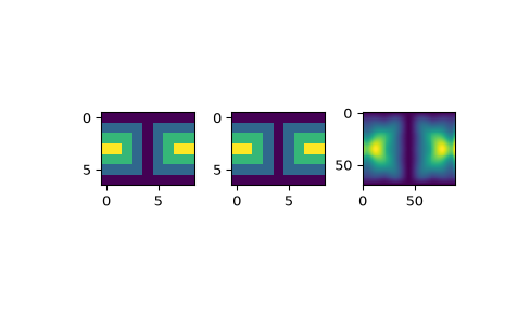
Suppose we have global data on a coarse grid (the input data does not have to be on a grid):

>>> from scipy.interpolate import LSQSphereBivariateSpline
>>> import numpy as np
>>> import matplotlib.pyplot as plt

>>> theta = np.linspace(0, np.pi, num=7)
>>> phi = np.linspace(0, 2*np.pi, num=9)
>>> data = np.empty((theta.shape[0], phi.shape[0]))
>>> data[:,0], data[0,:], data[-1,:] = 0., 0., 0.
>>> data[1:-1,1], data[1:-1,-1] = 1., 1.
>>> data[1,1:-1], data[-2,1:-1] = 1., 1.
>>> data[2:-2,2], data[2:-2,-2] = 2., 2.
>>> data[2,2:-2], data[-3,2:-2] = 2., 2.
>>> data[3,3:-2] = 3.
>>> data = np.roll(data, 4, 1)

We need to set up the interpolator object. Here, we must also specify the coordinates of the knots to use.

>>> lats, lons = np.meshgrid(theta, phi)
>>> knotst, knotsp = theta.copy(), phi.copy()
>>> knotst[0] += .0001
>>> knotst[-1] -= .0001
>>> knotsp[0] += .0001
>>> knotsp[-1] -= .0001
>>> lut = LSQSphereBivariateSpline(lats.ravel(), lons.ravel(),
...                                data.T.ravel(), knotst, knotsp)

As a first test, we’ll see what the algorithm returns when run on the input coordinates

>>> data_orig = lut(theta, phi)

Finally we interpolate the data to a finer grid

>>> fine_lats = np.linspace(0., np.pi, 70)
>>> fine_lons = np.linspace(0., 2*np.pi, 90)
>>> data_lsq = lut(fine_lats, fine_lons)

>>> fig = plt.figure()
>>> ax1 = fig.add_subplot(131)
>>> ax1.imshow(data, interpolation='nearest')
>>> ax2 = fig.add_subplot(132)
>>> ax2.imshow(data_orig, interpolation='nearest')
>>> ax3 = fig.add_subplot(133)
>>> ax3.imshow(data_lsq, interpolation='nearest')
>>> plt.show()

Go BackOpen In Tab