scipy.interpolate.

RectSphereBivariateSpline

class scipy.interpolate.RectSphereBivariateSpline(u, v, r, s=0.0, pole_continuity=False, pole_values=None, pole_exact=False, pole_flat=False)

Bivariate spline approximation over a rectangular mesh on a sphere.

Can be used for smoothing data.

Added in version 0.11.0.

Parameters:

uarray_like

1-D array of colatitude coordinates in strictly ascending order. Coordinates must be given in radians and lie within the open interval (0, pi).

varray_like

1-D array of longitude coordinates in strictly ascending order. Coordinates must be given in radians. First element (v[0]) must lie within the interval [-pi, pi). Last element (v[-1]) must satisfy v[-1] <= v[0] + 2*pi.

rarray_like

2-D array of data with shape (u.size, v.size).

sfloat, optional

Positive smoothing factor defined for estimation condition (s=0 is for interpolation).

pole_continuitybool or (bool, bool), optional

Order of continuity at the poles u=0 (pole_continuity[0]) and u=pi (pole_continuity[1]). The order of continuity at the pole will be 1 or 0 when this is True or False, respectively. Defaults to False.

pole_valuesfloat or (float, float), optional

Data values at the poles u=0 and u=pi. Either the whole parameter or each individual element can be None. Defaults to None.

pole_exactbool or (bool, bool), optional

Data value exactness at the poles u=0 and u=pi. If True, the value is considered to be the right function value, and it will be fitted exactly. If False, the value will be considered to be a data value just like the other data values. Defaults to False.

pole_flatbool or (bool, bool), optional

For the poles at u=0 and u=pi, specify whether or not the approximation has vanishing derivatives. Defaults to False.

Methods

__call__(theta, phi[, dtheta, dphi, grid])	Evaluate the spline or its derivatives at given positions.
ev(theta, phi[, dtheta, dphi])	Evaluate the spline at points
get_coeffs()	Return spline coefficients.
get_knots()	Return a tuple (tx,ty) where tx,ty contain knots positions of the spline with respect to x-, y-variable, respectively.
get_residual()	Return weighted sum of squared residuals of the spline approximation: sum ((w[i]*(z[i]-s(x[i],y[i])))**2,axis=0)
partial_derivative(dx, dy)	Construct a new spline representing a partial derivative of this spline.

See also

BivariateSpline

a base class for bivariate splines.

UnivariateSpline

a smooth univariate spline to fit a given set of data points.

SmoothBivariateSpline

a smoothing bivariate spline through the given points

LSQBivariateSpline

a bivariate spline using weighted least-squares fitting

SmoothSphereBivariateSpline

a smoothing bivariate spline in spherical coordinates

LSQSphereBivariateSpline

a bivariate spline in spherical coordinates using weighted least-squares fitting

RectBivariateSpline

a bivariate spline over a rectangular mesh.

bisplrep

a function to find a bivariate B-spline representation of a surface

bisplev

a function to evaluate a bivariate B-spline and its derivatives

Notes

Currently, only the smoothing spline approximation (iopt[0] = 0 and iopt[0] = 1 in the FITPACK routine) is supported. The exact least-squares spline approximation is not implemented yet.

When actually performing the interpolation, the requested v values must lie within the same length 2pi interval that the original v values were chosen from.

For more information, see the FITPACK site about this function.

Examples

Try it in your browser!

Suppose we have global data on a coarse grid

>>> import numpy as np
>>> lats = np.linspace(10, 170, 9) * np.pi / 180.
>>> lons = np.linspace(0, 350, 18) * np.pi / 180.
>>> data = np.dot(np.atleast_2d(90. - np.linspace(-80., 80., 18)).T,
...               np.atleast_2d(180. - np.abs(np.linspace(0., 350., 9)))).T

We want to interpolate it to a global one-degree grid

>>> new_lats = np.linspace(1, 180, 180) * np.pi / 180
>>> new_lons = np.linspace(1, 360, 360) * np.pi / 180
>>> new_lats, new_lons = np.meshgrid(new_lats, new_lons)

We need to set up the interpolator object

>>> from scipy.interpolate import RectSphereBivariateSpline
>>> lut = RectSphereBivariateSpline(lats, lons, data)

Finally we interpolate the data. The RectSphereBivariateSpline object only takes 1-D arrays as input, therefore we need to do some reshaping.

>>> data_interp = lut.ev(new_lats.ravel(),
...                      new_lons.ravel()).reshape((360, 180)).T

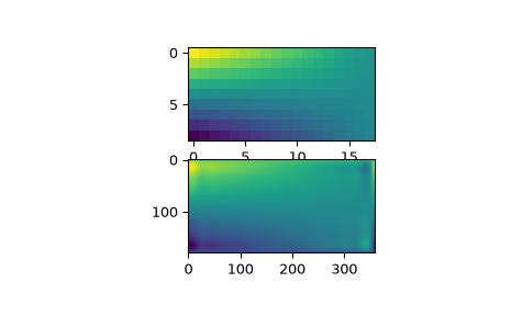
Looking at the original and the interpolated data, one can see that the interpolant reproduces the original data very well:

>>> import matplotlib.pyplot as plt
>>> fig = plt.figure()
>>> ax1 = fig.add_subplot(211)
>>> ax1.imshow(data, interpolation='nearest')
>>> ax2 = fig.add_subplot(212)
>>> ax2.imshow(data_interp, interpolation='nearest')
>>> plt.show()

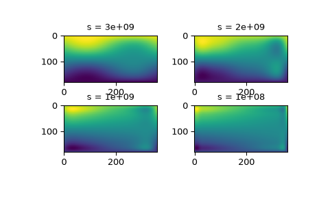
Choosing the optimal value of s can be a delicate task. Recommended values for s depend on the accuracy of the data values. If the user has an idea of the statistical errors on the data, she can also find a proper estimate for s. By assuming that, if she specifies the right s, the interpolator will use a spline f(u,v) which exactly reproduces the function underlying the data, she can evaluate sum((r(i,j)-s(u(i),v(j)))**2) to find a good estimate for this s. For example, if she knows that the statistical errors on her r(i,j)-values are not greater than 0.1, she may expect that a good s should have a value not larger than u.size * v.size * (0.1)**2.

If nothing is known about the statistical error in r(i,j), s must be determined by trial and error. The best is then to start with a very large value of s (to determine the least-squares polynomial and the corresponding upper bound fp0 for s) and then to progressively decrease the value of s (say by a factor 10 in the beginning, i.e. s = fp0 / 10, fp0 / 100, ... and more carefully as the approximation shows more detail) to obtain closer fits.

The interpolation results for different values of s give some insight into this process:

>>> fig2 = plt.figure()
>>> s = [3e9, 2e9, 1e9, 1e8]
>>> for idx, sval in enumerate(s, 1):
...     lut = RectSphereBivariateSpline(lats, lons, data, s=sval)
...     data_interp = lut.ev(new_lats.ravel(),
...                          new_lons.ravel()).reshape((360, 180)).T
...     ax = fig2.add_subplot(2, 2, idx)
...     ax.imshow(data_interp, interpolation='nearest')
...     ax.set_title(f"s = {sval:g}")
>>> plt.show()

Go BackOpen In Tab