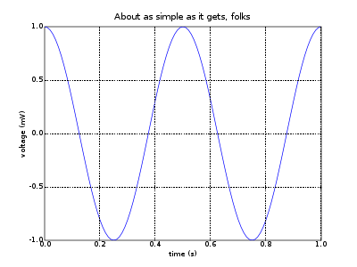
Matplotlib is the preferred 2D plotting library for Python users. The following is a collection of very simple programs from Matplotlib's examples directory. For powerful 3D plotting, see Mayavi.

For more examples you may want to check out the Matplotlib Cookbook and the official matplotlib tutorial at http://matplotlib.sf.net/tutorial.html.

Simple plot

   1 #!/usr/bin/env python
   2 """
   3 Example: simple line plot.
   4 Show how to make and save a simple line plot with labels, title and grid
   5 """
   6 import numpy
   7 import pylab
   8 
   9 t = numpy.arange(0.0, 1.0+0.01, 0.01)
  10 s = numpy.cos(2*2*numpy.pi*t)
  11 pylab.plot(t, s)
  12 
  13 pylab.xlabel('time (s)')
  14 pylab.ylabel('voltage (mV)')
  15 pylab.title('About as simple as it gets, folks')
  16 pylab.grid(True)
  17 pylab.savefig('simple_plot')
  18 
  19 pylab.show()

Image plot

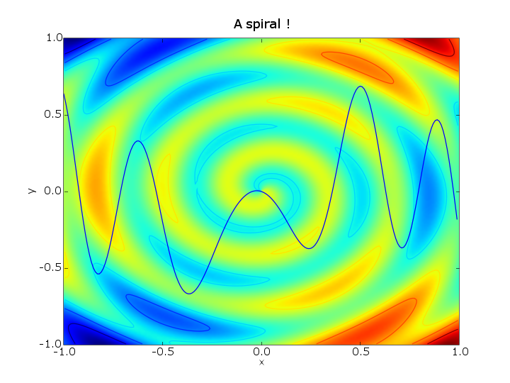
This small script shows two very useful things : how to display an image, i.e., a matrix of values, and how to plot contour lines, that is, lines following a constant value in the matrix. Using hold(True), we can overlay the two images, and in fact, any other line.

The imshow(z) method works by assigning a color to the values of the matrix z using a colormap. In the following example, the default colormap jet is used. The colormap basically consists of an index ranging from 0 to 1, to which rgb values are assigned. There exists a range of other colormaps similar to those in Matlab (TM), and it is not so difficult to create one from scratch. In the example, two options are passed with imshow : extent and origin. The extent argument simply tells matplotlib what the coordinates of the image are so it can label the x and y axis correctly. The origin option can take one of two values, 'upper' or 'lower'. The default is 'upper', which will just display the matrix as it is, with the (1,1) element in the upper left corner. With the 'lower' argument, the matrix is mirrored so the (1,1) element goes in the lower left corner. There are a lot more options to control imshow's behavior, such as cmap (colormap), norm (the normalization method), interpolation, alpha (transparency). With some tweaking, you'll get the result you want.

   1 # Formulas from C. Pickover
   2 
   3 from scipy import *
   4 from pylab import *
   5 
   6 # Creating the grid of coordinates x,y 
   7 x,y = ogrid[-1.:1.:.01, -1.:1.:.01]
   8 
   9 z = 3*y*(3*x**2-y**2)/4 + .5*cos(6*pi * sqrt(x**2 +y**2) + arctan2(x,y))
  10 
  11 hold(True)
  12 # Creating image
  13 imshow(z, origin='lower', extent=[-1,1,-1,1])
  14 
  15 # Plotting contour lines
  16 contour(z, origin='lower', extent=[-1,1,-1,1])
  17 
  18 xlabel('x')
  19 ylabel('y')
  20 title('A spiral !')
  21 
  22 # Adding a line plot slicing the z matrix just for fun. 
  23 plot(x[:], z[50, :])
  24 
  25 savefig('spiral')