Contents
Introduction
Naive but fairly general implementation of a Kalman Filter, together with some examples.
This program is based on the following paper:
- Greg Welch and Garry Bishop. An Introduction to the Kalman Filter.
See also:
A Kalman filter is an Algorithm to estimate the states of a linear dynamic system from noisy measurements. It must know the system's parameters, as well as the inputs, which may have process noise added to them.
System Equations:
xk = A xk-1 + B uk + wk(Q) |
(1) |
zk = H xk + vk(R) |
(2) |
with:
- x: State variables (vector)
- u: Inputs (vector)
- z: Outputs (vector)
- w: Random noise (vector) with covariance Q
- v: Random noise (vector) with covariance R
- A,B,H: Parameter matrices
Such a dynamic system can be interpreted as a system of linear differential equations, in a time discete form. Therfore the state variables of many physical systems can be estimated by a Kalman Filter. But there does not need to be an interpretation as a differential equation. Welsh and Bishop (the authors of the paper above) use the Kalman Filter to predict the position of moving objects in image sequences (IMHO).
As one can see from equation (2) it is not necessary to measure the state variables directly. A Kalman Filter can estimate the system states from a linear combination of them, with added noise. The Kalman filter does not need to store a long history of measurements. It stores only the current state estimate (xhat) and a matrix that specifies how much the filter trusts the current state estimate (P).
Structure of Program
The program (kalman.py) is fairly large (~1000 lines), however much space is taken by comments. First come some classes that do the maths:
LinSys: The dynamic system. Can simulate the system and generate the random noise. Needs all parameter matrices (A, B, H, Q, R) to run. Parent class for all example systems.
KalmanFilter: The Kalman filter. Needs a LinSys class to know the system's parameters.
PidController: A very simple PID controller.
Then come some example systems. These classes all inherit from LinSys. To create your own dynamic systems see the docstring of the LinSys class, and use one of the example systems as a starting point.
SysConstVal: In this system the state values simply stay constant.
SysTank: Tank with variable input and output.
SysSpringPendulum A damped spring pendulum. Forces are applied to pendulum's mass.
Finally there are several numerical experiments, which are described in the next section.
Numerical experiments
The numerical experiments are organized in (nested) functions. This way it is easy to enable/disable certain experiments by only commenting out the line where the experiment function is called.
SysConstVal Experiment
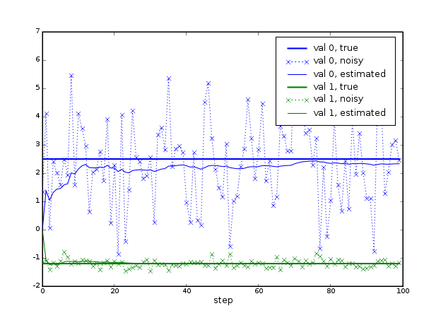
In this experiment the Kalman filter is asked to guess two constant values. The filter can only see the values with random noise (a random number) added to them. The filter is shown many such noisy measurements, and each time it is asked to estimate the true values. The noise for value 0 (blue) has a big variance, and the noise for value 1 (green) has a small variance. The filter knows the variances.

The filter behaves as an adaptable lowpass filter. When the noise's variance is big (blue) the filter does not trust the measurements very much, and the filter is slow to find the true value. When the noise's variance is small (green) it finds the true values quickly.
This experiment is very similar to the example in the paper mentioned in the introduction, and in the other Kalman Filtering example.
SysTank Experiment
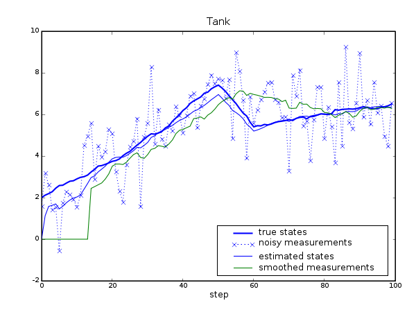
SysTank models a tank with variable inflow and outflow. The the amount of liquid in the tank is measured, but with a lot of noise added to it. The inflow and the outflow rates are known, and considerable process noise is added to them too. The Kalman filter is asked to estimate the amount of liquid in the tank.
For comparison a simple moving average filter is applied to the noisy measurements. It averages over 15 steps. As one can see in the image below, the Kalman filter performs significantly better than the averaging filter.

Program Code
Download the program:: kalman.py