#class right
## Snazzy graphics here...
[[ImageLink(mplscreenshotsm.png,Cookbook/OptimizationDemo1)]]
[:Cookbook/OptimizationDemo1: SciPy optimization example].
This page is intended to help the beginner get a handle on scipy and be productive with it as fast as possible.
Contents
What are scipy, numpy, matplotlib ?
Python is a general purpose programming language. It is interpreted and dynamically typed and is very suited for interactive work and quick prototyping, while being powerful enough to write large applications in.
Numpy is a language extension that defines the numerical array and matrix type and basic operations on them.
Scipy is another language extension that uses numpy to do advanced math, signal processing, optimization, statistics and much more.
Matplotlib is a language extension to facilitate plotting.
What are they useful for ?
Scipy and friends can be used for a variety of tasks:
- First of all, they are great for performing calculation relying heavily on mathematical and numerical operations. They can work natively with matrices and arrays, perform operations on them, find eigenvectors, compute integrals, solve differential equations.
Numpy's array class (which is used to implement the matrix class) is implemented with speed in mind, so accessing numpy arrays is faster than accessing Python lists. Further, numpy implements an array language, so that most loops are not needed. For example, Plain Python (and similarly for C, etc.):
a = range(10000000)
b = range(10000000)
c = []
for i in range(len(a)):
  c.append(a[i] + b[i])
import numpy as np
a = np.arange(10000000)
b = np.arange(10000000)
c = a + b
There is a sizeable collection of both generic and application-specific numerical code written in or using numpy and scipy. See the Topical Software index for a partial list. Python has many advanced modules to build interactive applications (for instance TraitsUI or wxPython). Using scipy with these is the quickest way to build a scientific application.
Using ipython makes interactive work easy. Data processing, exploration of numerical models, trying out operations on the fly allows to go quickly from an idea to a result (see the article on ipython).
The matplotlib module produces high quality plots. With it you can turn your data or your models into figures for presentations or articles. No need to do the numerical work in one program, save the data, and plot it with another program.
How to work with scipy
Python is a language, it comes with several user interfaces. There is no single program that you can start and that gives an integrated user experience. Instead of that there are dozens of way to work with python.
The most common is to use the advanced interactive python shell ipython to enter commands and run scripts. Scripts can be written with any text editor, for instance SPE, PyScripter, or even notepad, emacs, or vi.
Neither scipy nor numpy provide, by default, plotting functions. They are just numerical tools. The recommended plotting package is matplotlib.
Under Windows, Mac OS X, and Linux, all these tools are provided by the Enthought Python Distribution (http://www.enthought.com/products/epd.php), for more instruction on installing these see the Installing_SciPy section of this site.
Learning to use scipy
The quick way to get working with scipy is probably this tutorial focused on interactive data analysis.
To learn more about the python language, the python tutorial will make you familiar with the python syntax and objects. You can download this tutorial from http://docs.python.org/download.html .
Dave Kuhlman's course on numpy and scipy is another good introduction: http://www.rexx.com/~dkuhlman/scipy_course_01.html
The Documentation and Cookbook sections of this site provide more material for further learning.
An Example Session
Interactive work
Let's look at the Fourier transform of a square window. To do this we are going to use ipython, an interactive python shell. As we want to display our results with interactive plots, we will start ipython with the "-pylab" switch, which enables the interactive use of matplotlib.
$ ipython -pylab
Python 2.5.1 (r251:54863, May  2 2007, 16:27:44)
Type "copyright", "credits" or "license" for more information.
IPython 0.7.3 -- An enhanced Interactive Python.
?       -> Introduction to IPython's features.
%magic  -> Information about IPython's 'magic' % functions.
help    -> Python's own help system.
object? -> Details about 'object'. ?object also works, ?? prints more.
  Welcome to pylab, a matplotlib-based Python environment.
  For more information, type 'help(pylab)'.
Ipython offers a great many convenience features, such as tab-completion of python functions and a good help system.
In [1]: %logstart
Activating auto-logging. Current session state plus future input saved.
Filename       : ipython_log.py
Mode           : rotate
Output logging : False
Raw input log  : False
Timestamping   : False
State          : active
This activates logging of the session to a file. The format of the log file allows it to be simply executed as a python script at a later date, or edited into a program. Ipython also keeps track of all inputs and outputs (and makes them accessible in the lists called In and Out), so that you can start the logging retroactively.
In [2]: from scipy import *
Since numpy and scipy are not built into python, you must explicitly tell python to load their features. Scipy provides numpy so it is not necessary to import it when importing scipy.
Now to the actual math:
In [3]: a = zeros(1000)
In [4]: a[:100]=1
The first line simply makes an array of 1000 zeros, as you might expect; numpy defaults to making these zeros double-precision floating-point numbers, but if I had wanted single-precision or complex numbers, I could have specified an extra argument to zeros. The second line sets the first hundred entries to 1.
I next want to take the Fourier transform of this array. Scipy provides a fft function to do that:
In [5]: b = fft(a)
In order to see what b looks like, I'll use the matplotlib library. If you started ipython with the "-pylab" you do not need to import matplotlib. Elsewhere you can import it with: "from pylab import *", but you will not have interactive functionality (the plots displays as you create them).
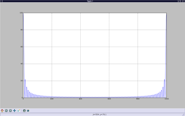
In [6]: plot(abs(b))
Out[6]: [<matplotlib.lines.Line2D instance at 0xb7b9144c>]
In [7]: show()

This brings up a window showing the graph of b. The show command on input "[7]" is not necessary if you started ipython with the "-pylab" switch.
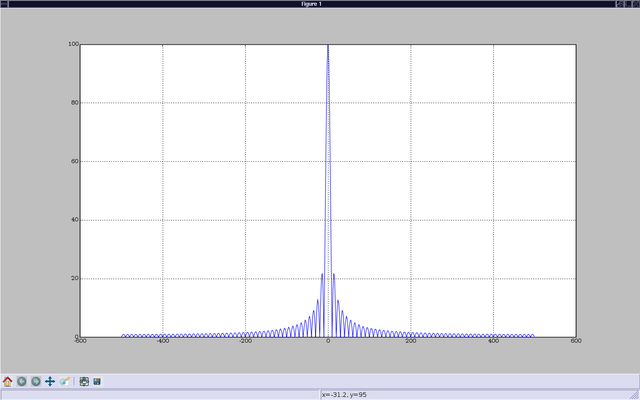
I notice that it would look nicer if I shifted b around to put zero frequency in the center. I can do this by concatenating the second half of b with the first half, but I don't quite remember the syntax for concatenate:
In [8]: concatenate?
Type:           builtin_function_or_method
Base Class:     <type 'builtin_function_or_method'>
String Form:    <built-in function concatenate>
Namespace:      Interactive
Docstring:
    concatenate((a1, a2, ...), axis=0)
    Join arrays together.
    The tuple of sequences (a1, a2, ...) are joined along the given axis
    (default is the first one) into a single numpy array.
    Example:
    >>> concatenate( ([0,1,2], [5,6,7]) )
    array([0, 1, 2, 5, 6, 7])
In [9]: f=arange(-500,500,1)
In [10]: grid(True)
In [11]: plot(f,abs(concatenate((b[500:],b[:500]))))
Out[11]: [<matplotlib.lines.Line2D instance at 0xb360ca4c>]
In [12]: show()
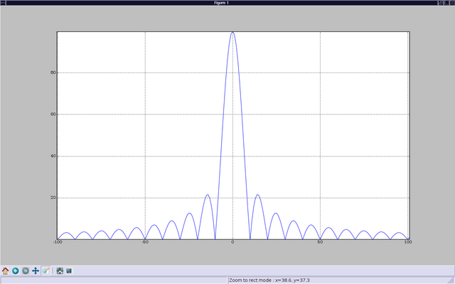
This brings up the graph I wanted. I can also pan and zoom, using a set of interactive controls, and generate postscript output for inclusion in publications (If you want to learn more about plotting, you are advised to read the matplotlib tutorial).

Running a script
When you are repeating the same work over and over, it can be useful to save the commands in a file and run it as a script in ipython. You can quit the current ipython session using "ctrl-D" and edit the file ipython_log.py. When you want to execute the instructions in this file you can open a new ipython session an enter the command "%run -i ipython_log.py".
It can also be handy to try out a few commands in ipython, while editing a script file. This allows to try the script line by line on some simple cases before saving it and running it.
Some notes about importing
The following is not so important for you if you are just about to start with scipy & friends and you shouldn't worry about it. But it's good to keep it in mind when you start to develop some larger applications.
For interactive work (in ipython) and for smaller scripts it's ok to use from scipy import *. This has the advantage of having all functionallity in the current namespace ready to go. However, for larger programs/packages it is advised to import only the functions or modules that you really need. Lets consider the case where you (for whatever reason) want to compare numpy's and scipy's fft functions. In your script you would then write
# import from module numpy.fft
from numpy.fft import fft
# import scipy's fft implementation and rename it;
# Note: `from scipy import fft` actually imports numpy.fft.fft (check with
# `scipy.fft?` in Ipython or look at .../site-packages/scipy/__init__.py)
from scipy.fftpack import fft as scipy_fft
The advantage is that you can, when looking at your code, see explicitly what you are importing, which results in clear and readable code. Additionally, this is often faster than importing everything with import *, especially if you import from a rather large package like scipy.
However, if you use many different numpy functions, the import statement would get very long if you import everything explicitly. But instead of using import * you can import the whole package.
from numpy import *  # bad
from numpy import abs, concatenate, sin, pi, dot, amin, amax, asarray, cov, diag, zeros, empty, exp, eye, kaiser # very long
import numpy         # good
# use numpy.fft.fft() on array 'a'
b = numpy.fft.fft(a)
This is ok since usually import numpy is quite fast. Scipy, on the other hand, is rather big (has many subpackages). Therefore, from scipy import * can be slow on the first import (all subsequent import statements will be executed faster because no re-import is actually done). That's why the importing of subpackages (like scipy.fftpack) is disabled by default if you say import scipy, which then is as fast as import numpy. If you want to use, say scipy.fftpack, you have to import it explicitly (which is a good idea anyway). If you want to load all scipy subpackges at once, you will have to do import scipy; scipy.pkgload(). For interactive sessions with Ipython, you can invoke it with the scipy profile (ipython -p scipy), which reads the scipy profile rc file (usually ~/.ipython/ipythonrc-scipy) and loads all of scipy for you. For a ready-to-go interactive environment with scipy and matplotlib plotting, you would use something like ipython -pylab -p scipy.
For a general overview of package structuring and "pythonic" importing conventions, take a look at this part of the Python tutorial.