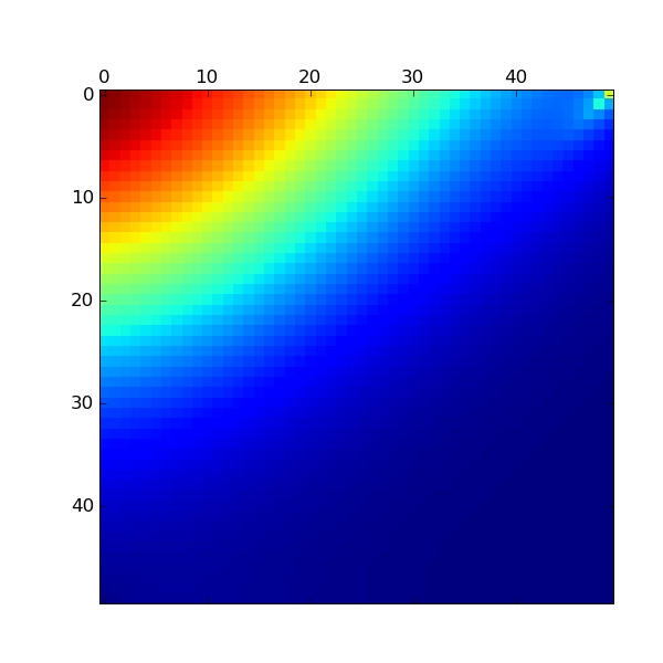
This page shows how to compute the stationary distribution pi of a large Markov chain. The example is a tandem of two M/M/1 queues. Generally the transition matrix P of the Markov chain is sparse, so that we can either use scipy.sparse or Pysparse. Here we demonstrate how to use both of these tools.
Power Method
In this section we find pi by means of iterative methods called the Power method. More specifically, given a (stochastic) transition matrix P, and an initial vector pi_0, compute iteratively pi_n = pi_{n-1} P until the distance (in some norm) between pi_n and pi_{n-1} is small enough.
Fist we build the generator matrix Q for the related Markov chain. Then we turn Q into a transition matrix P by the method of uniformization, that is, we define P as I - Q/l, where I is the identity matrix (of the same size as Q) and l is the smallest element on the diagonal of Q. Once we have P, we approximate pi (the left eigenvector of P that satisfies pi = pi P) by the iterates pi_n = pi_0 P^n, for some initial vector pi_0.
More details of the above approach can be found in (more or less) any book on probability and Markov Chains. A fine example, with many nice examples and attention to the numerical solution of Markov chains, is `Queueing networks and Markov Chains' by G. Bolch et al., John Wiley, 2nd edition, 2006.
You can get the source code for this tutorial here: tandemqueue.py
This simple function converts the state (i,j), which represents that the first queue contains i jobs and the second queue j jobs, to a more suitable form to define a transition matrix.
Build the off-diagonal elements of the generator matrix Q.
   1 def fillOffDiagonal(Q):
   2     # labda
   3     for i in range(0,N1-1):
   4         for j in range(0,N2):
   5             Q[(state(i,j),state(i+1,j))]= labda
   6     # mu2
   7     for i in range(0,N1):
   8         for j in range(1,N2):
   9             Q[(state(i,j),state(i,j-1))]= mu2
  10     # mu1
  11     for i in range(1,N1):
  12         for j in range(0,N2-1):
  13             Q[(state(i,j),state(i-1,j+1))]= mu1
  14     print "ready filling"
In this function we use scipy.sparse
   1 def computePiMethod1():
   2     e0 = time.time()
   3     Q = sp.dok_matrix((size,size))
   4     fillOffDiagonal(Q)
   5     # Set the diagonal of Q such that the row sums are zero
   6     Q.setdiag( -Q*ones(size) )
   7     # Compute a suitable stochastic matrix by means of uniformization
   8     l = min(Q.values())*1.001  # avoid periodicity, see the book of Bolch et al.
   9     P = sp.speye(size, size) - Q/l
  10     # compute Pi
  11     P =  P.tocsr()
  12     pi = zeros(size);  pi1 = zeros(size)
  13     pi[0] = 1;
  14     n = norm(pi - pi1,1); i = 0;
  15     while n > 1e-3 and i < 1e5:
  16         pi1 = pi*P
  17         pi = pi1*P   # avoid copying pi1 to pi
  18         n = norm(pi - pi1,1); i += 1
  19     print "Method 1: ", time.time() - e0, i
  20     return pi
Now use Pysparse.
   1 def computePiMethod2():
   2     e0 = time.time()
   3     Q = pysparse.spmatrix.ll_mat(size,size)
   4     fillOffDiagonal(Q)
   5     # fill diagonal
   6     x =  empty(size)
   7     Q.matvec(ones(size),x)
   8     Q.put(-x)
   9     # uniformize
  10     l = min(Q.values())*1.001
  11     P = pysparse.spmatrix.ll_mat(size,size)
  12     P.put(ones(size))
  13     P.shift(-1./l, Q)
  14     # Compute pi
  15     P = P.to_csr()
  16     pi = zeros(size);  pi1 = zeros(size)
  17     pi[0] = 1;
  18     n = norm(pi - pi1,1); i = 0;
  19     while n > 1e-3 and i < 1e5:
  20         P.matvec_transp(pi,pi1)
  21         P.matvec_transp(pi1,pi)
  22         n = norm(pi - pi1,1); i += 1
  23     print "Method 2: ", time.time() - e0, i
  24     return pi
Output the results.
Here is the result:
Improvements of this Tutorial
Include other methods such as Jacobi's method or Gauss Seidel.
