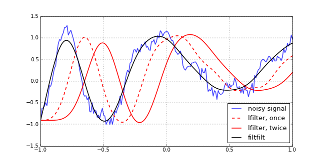
This sample code demonstrates the use of the function scipy.signal.filtfilt, a linear filter that achieves zero phase delay by applying an IIR filter to a signal twice, once forwards and once backwards. The order of the filter is twice the original filter order. The function also computes the initial filter parameters in order to provide a more stable response (via lfilter_zi).
For comparison, this script also applies the same IIR filter to the signal using scipy.signal.lfilter; for these calculations, lfilter_zi is used to choose appropriate initial conditions for the filter. Without this, these plots would have long transients near 0. As it is, they have long transients near the initial value of the signal.
Code
   1 from numpy import sin, cos, pi, linspace
   2 from numpy.random import randn
   3 from scipy.signal import lfilter, lfilter_zi, filtfilt, butter
   4
   5 from matplotlib.pyplot import plot, legend, show, hold, grid, figure, savefig
   6
   7
   8 # Generate a noisy signal to be filtered.
   9 t = linspace(-1, 1, 201)
  10 x = (sin(2 * pi * 0.75 * t*(1-t) + 2.1) + 0.1*sin(2 * pi * 1.25 * t + 1) +
  11     0.18*cos(2 * pi * 3.85 * t))
  12 xn = x + randn(len(t)) * 0.08
  13
  14 # Create an order 3 lowpass butterworth filter.
  15 b, a = butter(3, 0.05)
  16
  17 # Apply the filter to xn.  Use lfilter_zi to choose the initial condition
  18 # of the filter.
  19 zi = lfilter_zi(b, a)
  20 z, _ = lfilter(b, a, xn, zi=zi*xn[0])
  21
  22 # Apply the filter again, to have a result filtered at an order
  23 # the same as filtfilt.
  24 z2, _ = lfilter(b, a, z, zi=zi*z[0])
  25
  26 # Use filtfilt to apply the filter.
  27 y = filtfilt(b, a, xn)
  28
  29
  30 # Make the plot.
  31 figure(figsize=(10,5))
  32 hold(True)
  33 plot(t, xn, 'b', linewidth=1.75, alpha=0.75)
  34 plot(t, z, 'r--', linewidth=1.75)
  35 plot(t, z2, 'r', linewidth=1.75)
  36 plot(t, y, 'k', linewidth=1.75)
  37 legend(('noisy signal',
  38         'lfilter, once',
  39         'lfilter, twice',
  40         'filtfilt'),
  41         loc='best')
  42 hold(False)
  43 grid(True)
  44 show()
  45 #savefig('plot.png', dpi=65)
Figure
