Brownian Motion
Brownian motion is a stochastic process. One form of the equation for Brownian motion is
X(0) = X0
X(t + dt) = X(t) + N(0, (delta)2 dt; t, t+dt)
where N(a, b; t1, t2) is a normally distributed random variable with mean a and variance b. The parameters t1 and t2 make explicit the statistical independence of N on different time intervals; that is, if [t1, t2) and [t3, t4) are disjoint intervals, then N(a, b; t1, t2) and N(a, b; t3, t4) are independent.
The calculation is actually very simple. A naive implementation that prints n steps of the Brownian motion might look like this:
The above code could be easily modified to save the iterations in an array instead of printing them.
The problem with the above code is that it is slow. If we want to compute a large number of iterations, we can do much better. The key is to note that the calculation is the cumulative sum of samples from the normal distribution. A fast version can be implemented by first generating all the samples from the normal distribution with one call to scipy.stats.norm.rvs(), and then using the numpy cumsum function to form the cumulative sum.
The following function uses this idea to implement the function brownian(). The function allows the initial condition to be an array (or anything that can be converted to an array). Each element of x0 is treated as an initial condition for a Brownian motion.
   1 """
   2 brownian() implements one dimensional Brownian motion (i.e. the Wiener process).
   3 """
   4
   5 # File: brownian.py
   6
   7 from math import sqrt
   8 from scipy.stats import norm
   9 import numpy as np
  10
  11
  12 def brownian(x0, n, dt, delta, out=None):
  13     """\
  14     Generate an instance of Brownian motion (i.e. the Wiener process):
  15
  16         X(t) = X(0) + N(0, delta**2 * t; 0, t)
  17
  18     where N(a,b; t0, t1) is a normally distributed random variable with mean a and
  19     variance b.  The parameters t0 and t1 make explicit the statistical
  20     independence of N on different time intervals; that is, if [t0, t1) and
  21     [t2, t3) are disjoint intervals, then N(a, b; t0, t1) and N(a, b; t2, t3)
  22     are independent.
  23
  24     Written as an iteration scheme,
  25
  26         X(t + dt) = X(t) + N(0, delta**2 * dt; t, t+dt)
  27
  28
  29     If `x0` is an array (or array-like), each value in `x0` is treated as
  30     an initial condition, and the value returned is a numpy array with one
  31     more dimension than `x0`.
  32
  33     Arguments
  34     ---------
  35     x0 : float or numpy array (or something that can be converted to a numpy array
  36          using numpy.asarray(x0)).
  37         The initial condition(s) (i.e. position(s)) of the Brownian motion.
  38     n : int
  39         The number of steps to take.
  40     dt : float
  41         The time step.
  42     delta : float
  43         delta determines the "speed" of the Brownian motion.  The random variable
  44         of the position at time t, X(t), has a normal distribution whose mean is
  45         the position at time t=0 and whose variance is delta**2*t.
  46     out : numpy array or None
  47         If `out` is not None, it specifies the array in which to put the
  48         result.  If `out` is None, a new numpy array is created and returned.
  49
  50     Returns
  51     -------
  52     A numpy array of floats with shape `x0.shape + (n,)`.
  53
  54     Note that the initial value `x0` is not included in the returned array.
  55     """
  56
  57     x0 = np.asarray(x0)
  58
  59     # For each element of x0, generate a sample of n numbers from a
  60     # normal distribution.
  61     r = norm.rvs(size=x0.shape + (n,), scale=delta*sqrt(dt))
  62
  63     # If `out` was not given, create an output array.
  64     if out is None:
  65         out = np.empty(r.shape)
  66
  67     # This computes the Brownian motion by forming the cumulative sum of
  68     # the random samples.
  69     np.cumsum(r, axis=-1, out=out)
  70
  71     # Add the initial condition.
  72     out += np.expand_dims(x0, axis=-1)
  73
  74     return out
Example
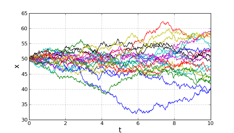
Here's a script that uses this function and matplotlib's pylab module to plot several realizations of Brownian motion.
   1 import numpy
   2 from pylab import plot, show, grid, xlabel, ylabel
   3
   4 from brownian import brownian
   5
   6
   7 def main():
   8
   9     # The Wiener process parameter.
  10     delta = 2
  11     # Total time.
  12     T = 10.0
  13     # Number of steps.
  14     N = 500
  15     # Time step size
  16     dt = T/N
  17     # Number of realizations to generate.
  18     m = 20
  19     # Create an empty array to store the realizations.
  20     x = numpy.empty((m,N+1))
  21     # Initial values of x.
  22     x[:, 0] = 50
  23
  24     brownian(x[:,0], N, dt, delta, out=x[:,1:])
  25
  26     t = numpy.linspace(0.0, N*dt, N+1)
  27     for k in range(m):
  28         plot(t, x[k])
  29     xlabel('t', fontsize=16)
  30     ylabel('x', fontsize=16)
  31     grid(True)
  32     show()
  33
  34
  35 if __name__ == "__main__":
  36     main()
The following shows a typical plot generated by the script.

2D Brownian Motion
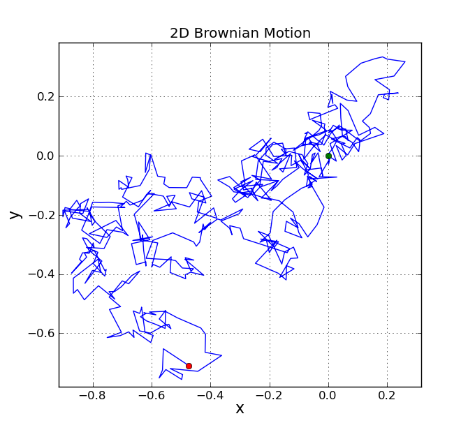
The same function can be used to generate Brownian motion in two dimensions, since each dimension is just a one-dimensional Brownian motion.
The following script provides a demo.
   1 import numpy
   2 from pylab import plot, show, grid, axis, xlabel, ylabel, title
   3
   4 from brownian import brownian
   5
   6
   7 def main():
   8
   9     # The Wiener process parameter.
  10     delta = 0.25
  11     # Total time.
  12     T = 10.0
  13     # Number of steps.
  14     N = 500
  15     # Time step size
  16     dt = T/N
  17     # Initial values of x.
  18     x = numpy.empty((2,N+1))
  19     x[:, 0] = 0.0
  20
  21     brownian(x[:,0], N, dt, delta, out=x[:,1:])
  22
  23     # Plot the 2D trajectory.
  24     plot(x[0],x[1])
  25
  26     # Mark the start and end points.
  27     plot(x[0,0],x[1,0], 'go')
  28     plot(x[0,-1], x[1,-1], 'ro')
  29
  30     # More plot decorations.
  31     title('2D Brownian Motion')
  32     xlabel('x', fontsize=16)
  33     ylabel('y', fontsize=16)
  34     axis('equal')
  35     grid(True)
  36     show()
  37
  38
  39 if __name__ == "__main__":
  40     main()
A typical plot generated by this script is shown below.
