PoissonDisk#
- class scipy.stats.qmc.PoissonDisk(d, *, radius=0.05, hypersphere='volume', ncandidates=30, optimization=None, rng=None, l_bounds=None, u_bounds=None, seed=None)[source]#
Poisson disk sampling.
- Parameters:
- dint
Dimension of the parameter space.
- radiusfloat
Minimal distance to keep between points when sampling new candidates.
- hypersphere{“volume”, “surface”}, optional
Sampling strategy to generate potential candidates to be added in the final sample. Default is “volume”.
volume: original Bridson algorithm as described in [1]. New candidates are sampled within the hypersphere.surface: only sample the surface of the hypersphere.
- ncandidatesint
Number of candidates to sample per iteration. More candidates result in a denser sampling as more candidates can be accepted per iteration.
- optimization{None, “random-cd”, “lloyd”}, optional
Whether to use an optimization scheme to improve the quality after sampling. Note that this is a post-processing step that does not guarantee that all properties of the sample will be conserved. Default is None.
random-cd: random permutations of coordinates to lower the centered discrepancy. The best sample based on the centered discrepancy is constantly updated. Centered discrepancy-based sampling shows better space-filling robustness toward 2D and 3D subprojections compared to using other discrepancy measures.lloyd: Perturb samples using a modified Lloyd-Max algorithm. The process converges to equally spaced samples.
Added in version 1.10.0.
- rng
numpy.random.Generator, optional Pseudorandom number generator state. When rng is None, a new
numpy.random.Generatoris created using entropy from the operating system. Types other thannumpy.random.Generatorare passed tonumpy.random.default_rngto instantiate aGenerator.Changed in version 1.15.0: As part of the SPEC-007 transition from use of
numpy.random.RandomStatetonumpy.random.Generator, this keyword was changed from seed to rng. For an interim period, both keywords will continue to work, although only one may be specified at a time. After the interim period, function calls using the seed keyword will emit warnings. Following a deprecation period, the seed keyword will be removed.- l_bounds, u_boundsarray_like (d,)
Lower and upper bounds of target sample data.
Methods
fast_forward(n)Fast-forward the sequence by n positions.
Draw
nsamples in the interval[l_bounds, u_bounds].integers(l_bounds, *[, u_bounds, n, ...])Draw n integers from l_bounds (inclusive) to u_bounds (exclusive), or if endpoint=True, l_bounds (inclusive) to u_bounds (inclusive).
random([n, workers])Draw n in the half-open interval
[0, 1).reset()Reset the engine to base state.
Notes
Poisson disk sampling is an iterative sampling strategy. Starting from a seed sample, ncandidates are sampled in the hypersphere surrounding the seed. Candidates below a certain radius or outside the domain are rejected. New samples are added in a pool of sample seed. The process stops when the pool is empty or when the number of required samples is reached.
The maximum number of point that a sample can contain is directly linked to the radius. As the dimension of the space increases, a higher radius spreads the points further and help overcome the curse of dimensionality. See the quasi monte carlo tutorial for more details.
Warning
The algorithm is more suitable for low dimensions and sampling size due to its iterative nature and memory requirements. Selecting a small radius with a high dimension would mean that the space could contain more samples than using lower dimension or a bigger radius.
Some code taken from [2], written consent given on 31.03.2021 by the original author, Shamis, for free use in SciPy under the 3-clause BSD.
References
Examples
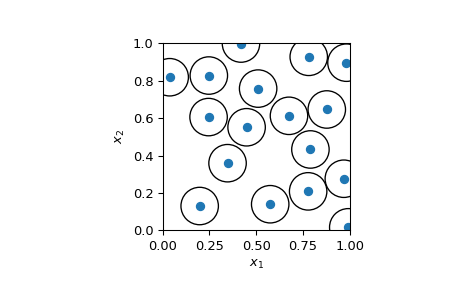
Generate a 2D sample using a radius of 0.2.
>>> import numpy as np
>>> import matplotlib.pyplot as plt
>>> from matplotlib.collections import PatchCollection
>>> from scipy.stats import qmc
>>>
>>> rng = np.random.default_rng()
>>> radius = 0.2
>>> engine = qmc.PoissonDisk(d=2, radius=radius, rng=rng)
>>> sample = engine.random(20)
Visualizing the 2D sample and showing that no points are closer than radius.
radius/2is used to visualize non-intersecting circles. If two samples are exactly at radius from each other, then their circle of radiusradius/2will touch.>>> fig, ax = plt.subplots() >>> _ = ax.scatter(sample[:, 0], sample[:, 1]) >>> circles = [plt.Circle((xi, yi), radius=radius/2, fill=False) ... for xi, yi in sample] >>> collection = PatchCollection(circles, match_original=True) >>> ax.add_collection(collection) >>> _ = ax.set(aspect='equal', xlabel=r'$x_1$', ylabel=r'$x_2$', ... xlim=[0, 1], ylim=[0, 1]) >>> plt.show()

Such visualization can be seen as circle packing: how many circle can we put in the space. It is an np-hard problem. The method
fill_spacecan be used to add samples until no more samples can be added. This is a hard problem and parameters may need to be adjusted manually. Beware of the dimension: as the dimensionality increases, the number of samples required to fill the space increases exponentially (curse-of-dimensionality).