scipy.stats.power

scipy.stats.power(test, rvs, n_observations, *, significance=0.01, vectorized=None, n_resamples=10000, batch=None, kwargs=None)

Simulate the power of a hypothesis test under an alternative hypothesis.

Parameters:

testcallable

Hypothesis test for which the power is to be simulated. test must be a callable that accepts a sample (e.g. test(sample)) or len(rvs) separate samples (e.g. test(samples1, sample2) if rvs contains two callables and n_observations contains two values) and returns the p-value of the test. If vectorized is set to True, test must also accept a keyword argument axis and be vectorized to perform the test along the provided axis of the samples. Any callable from scipy.stats with an axis argument that returns an object with a pvalue attribute is also acceptable.

rvscallable or tuple of callables

A callable or sequence of callables that generate(s) random variates under the alternative hypothesis. Each element of rvs must accept keyword argument size (e.g. rvs(size=(m, n))) and return an N-d array of that shape. If rvs is a sequence, the number of callables in rvs must match the number of elements of n_observations, i.e. len(rvs) == len(n_observations). If rvs is a single callable, n_observations is treated as a single element.

n_observationstuple of ints or tuple of integer arrays

If a sequence of ints, each is the sizes of a sample to be passed to test. If a sequence of integer arrays, the power is simulated for each set of corresponding sample sizes. See Examples.

significancefloat or array_like of floats, default: 0.01

The threshold for significance; i.e., the p-value below which the hypothesis test results will be considered as evidence against the null hypothesis. Equivalently, the acceptable rate of Type I error under the null hypothesis. If an array, the power is simulated for each significance threshold.

kwargsdict, optional

Keyword arguments to be passed to rvs and/or test callables. Introspection is used to determine which keyword arguments may be passed to each callable. The value corresponding with each keyword must be an array. Arrays must be broadcastable with one another and with each array in n_observations. The power is simulated for each set of corresponding sample sizes and arguments. See Examples.

vectorizedbool, optional

If vectorized is set to False, test will not be passed keyword argument axis and is expected to perform the test only for 1D samples. If True, test will be passed keyword argument axis and is expected to perform the test along axis when passed N-D sample arrays. If None (default), vectorized will be set True if axis is a parameter of test. Use of a vectorized test typically reduces computation time.

n_resamplesint, default: 10000

Number of samples drawn from each of the callables of rvs. Equivalently, the number tests performed under the alternative hypothesis to approximate the power.

batchint, optional

The number of samples to process in each call to test. Memory usage is proportional to the product of batch and the largest sample size. Default is None, in which case batch equals n_resamples.

Returns:

resPowerResult

An object with attributes:

powerfloat or ndarray

The estimated power against the alternative.

pvaluesndarray

The p-values observed under the alternative hypothesis.

Notes

The power is simulated as follows:

• Draw many random samples (or sets of samples), each of the size(s) specified by n_observations, under the alternative specified by rvs.

• For each sample (or set of samples), compute the p-value according to test. These p-values are recorded in the pvalues attribute of the result object.

• Compute the proportion of p-values that are less than the significance level. This is the power recorded in the power attribute of the result object.

Suppose that significance is an array with shape shape1, the elements of kwargs and n_observations are mutually broadcastable to shape shape2, and test returns an array of p-values of shape shape3. Then the result object power attribute will be of shape shape1 + shape2 + shape3, and the pvalues attribute will be of shape shape2 + shape3 + (n_resamples,).

Examples

Try it in your browser!

Suppose we wish to simulate the power of the independent sample t-test under the following conditions:

• The first sample has 10 observations drawn from a normal distribution with mean 0.

• The second sample has 12 observations drawn from a normal distribution with mean 1.0.

• The threshold on p-values for significance is 0.05.

>>> import numpy as np
>>> from scipy import stats
>>> rng = np.random.default_rng()
>>>
>>> test = stats.ttest_ind
>>> n_observations = (10, 12)
>>> rvs1 = rng.normal
>>> rvs2 = lambda size: rng.normal(loc=1, size=size)
>>> rvs = (rvs1, rvs2)
>>> res = stats.power(test, rvs, n_observations, significance=0.05)
>>> res.power
0.6116

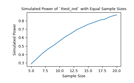
With samples of size 10 and 12, respectively, the power of the t-test with a significance threshold of 0.05 is approximately 60% under the chosen alternative. We can investigate the effect of sample size on the power by passing sample size arrays.

>>> import matplotlib.pyplot as plt
>>> nobs_x = np.arange(5, 21)
>>> nobs_y = nobs_x
>>> n_observations = (nobs_x, nobs_y)
>>> res = stats.power(test, rvs, n_observations, significance=0.05)
>>> ax = plt.subplot()
>>> ax.plot(nobs_x, res.power)
>>> ax.set_xlabel('Sample Size')
>>> ax.set_ylabel('Simulated Power')
>>> ax.set_title('Simulated Power of `ttest_ind` with Equal Sample Sizes')
>>> plt.show()

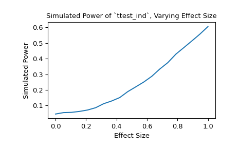
Alternatively, we can investigate the impact that effect size has on the power. In this case, the effect size is the location of the distribution underlying the second sample.

>>> n_observations = (10, 12)
>>> loc = np.linspace(0, 1, 20)
>>> rvs2 = lambda size, loc: rng.normal(loc=loc, size=size)
>>> rvs = (rvs1, rvs2)
>>> res = stats.power(test, rvs, n_observations, significance=0.05,
...                   kwargs={'loc': loc})
>>> ax = plt.subplot()
>>> ax.plot(loc, res.power)
>>> ax.set_xlabel('Effect Size')
>>> ax.set_ylabel('Simulated Power')
>>> ax.set_title('Simulated Power of `ttest_ind`, Varying Effect Size')
>>> plt.show()

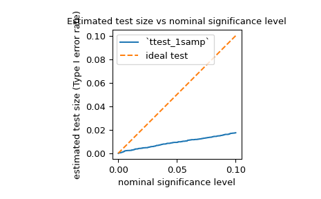
We can also use power to estimate the Type I error rate (also referred to by the ambiguous term “size”) of a test and assess whether it matches the nominal level. For example, the null hypothesis of jarque_bera is that the sample was drawn from a distribution with the same skewness and kurtosis as the normal distribution. To estimate the Type I error rate, we can consider the null hypothesis to be a true alternative hypothesis and calculate the power.

>>> test = stats.jarque_bera
>>> n_observations = 10
>>> rvs = rng.normal
>>> significance = np.linspace(0.0001, 0.1, 1000)
>>> res = stats.power(test, rvs, n_observations, significance=significance)
>>> size = res.power

As shown below, the Type I error rate of the test is far below the nominal level for such a small sample, as mentioned in its documentation.

>>> ax = plt.subplot()
>>> ax.plot(significance, size)
>>> ax.plot([0, 0.1], [0, 0.1], '--')
>>> ax.set_xlabel('nominal significance level')
>>> ax.set_ylabel('estimated test size (Type I error rate)')
>>> ax.set_title('Estimated test size vs nominal significance level')
>>> ax.set_aspect('equal', 'box')
>>> ax.legend(('`ttest_1samp`', 'ideal test'))
>>> plt.show()

As one might expect from such a conservative test, the power is quite low with respect to some alternatives. For example, the power of the test under the alternative that the sample was drawn from the Laplace distribution may not be much greater than the Type I error rate.

>>> rvs = rng.laplace
>>> significance = np.linspace(0.0001, 0.1, 1000)
>>> res = stats.power(test, rvs, n_observations, significance=0.05)
>>> print(res.power)
0.0587

This is not a mistake in SciPy’s implementation; it is simply due to the fact that the null distribution of the test statistic is derived under the assumption that the sample size is large (i.e. approaches infinity), and this asymptotic approximation is not accurate for small samples. In such cases, resampling and Monte Carlo methods (e.g. permutation_test, goodness_of_fit, monte_carlo_test) may be more appropriate.

Go BackOpen In Tab