scipy.stats.ecdf

scipy.stats.ecdf(sample)

Empirical cumulative distribution function of a sample.

The empirical cumulative distribution function (ECDF) is a step function estimate of the CDF of the distribution underlying a sample. This function returns objects representing both the empirical distribution function and its complement, the empirical survival function.

Parameters:

sample1D array_like or scipy.stats.CensoredData

Besides array_like, instances of scipy.stats.CensoredData containing uncensored and right-censored observations are supported. Currently, other instances of scipy.stats.CensoredData will result in a NotImplementedError.

Returns:

resECDFResult

An object with the following attributes.

cdfEmpiricalDistributionFunction

An object representing the empirical cumulative distribution function.

sfEmpiricalDistributionFunction

An object representing the empirical survival function.

The cdf and sf attributes themselves have the following attributes.

quantilesndarray

The unique values in the sample that defines the empirical CDF/SF.

probabilitiesndarray

The point estimates of the probabilities corresponding with quantiles.

And the following methods:

evaluate(x) :

Evaluate the CDF/SF at the argument.

plot(ax) :

Plot the CDF/SF on the provided axes.

confidence_interval(confidence_level=0.95) :

Compute the confidence interval around the CDF/SF at the values in quantiles.

Notes

When each observation of the sample is a precise measurement, the ECDF steps up by 1/len(sample) at each of the observations [1].

When observations are lower bounds, upper bounds, or both upper and lower bounds, the data is said to be “censored”, and sample may be provided as an instance of scipy.stats.CensoredData.

For right-censored data, the ECDF is given by the Kaplan-Meier estimator [2]; other forms of censoring are not supported at this time.

Confidence intervals are computed according to the Greenwood formula or the more recent “Exponential Greenwood” formula as described in [4].

References

[1] (1,2,3)

Conover, William Jay. Practical nonparametric statistics. Vol. 350. John Wiley & Sons, 1999.

[2]

Kaplan, Edward L., and Paul Meier. “Nonparametric estimation from incomplete observations.” Journal of the American statistical association 53.282 (1958): 457-481.

[3]

Goel, Manish Kumar, Pardeep Khanna, and Jugal Kishore. “Understanding survival analysis: Kaplan-Meier estimate.” International journal of Ayurveda research 1.4 (2010): 274.

[4]

Sawyer, Stanley. “The Greenwood and Exponential Greenwood Confidence Intervals in Survival Analysis.” https://www.math.wustl.edu/~sawyer/handouts/greenwood.pdf

Examples

Try it in your browser!

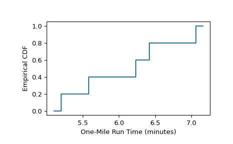
Uncensored Data

As in the example from [1] page 79, five boys were selected at random from those in a single high school. Their one-mile run times were recorded as follows.

>>> sample = [6.23, 5.58, 7.06, 6.42, 5.20]  # one-mile run times (minutes)

The empirical distribution function, which approximates the distribution function of one-mile run times of the population from which the boys were sampled, is calculated as follows.

>>> from scipy import stats
>>> res = stats.ecdf(sample)
>>> res.cdf.quantiles
array([5.2 , 5.58, 6.23, 6.42, 7.06])
>>> res.cdf.probabilities
array([0.2, 0.4, 0.6, 0.8, 1. ])

To plot the result as a step function:

>>> import matplotlib.pyplot as plt
>>> ax = plt.subplot()
>>> res.cdf.plot(ax)
>>> ax.set_xlabel('One-Mile Run Time (minutes)')
>>> ax.set_ylabel('Empirical CDF')
>>> plt.show()

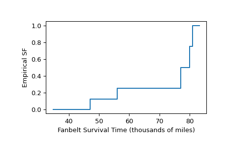
Right-censored Data

As in the example from [1] page 91, the lives of ten car fanbelts were tested. Five tests concluded because the fanbelt being tested broke, but the remaining tests concluded for other reasons (e.g. the study ran out of funding, but the fanbelt was still functional). The mileage driven with the fanbelts were recorded as follows.

>>> broken = [77, 47, 81, 56, 80]  # in thousands of miles driven
>>> unbroken = [62, 60, 43, 71, 37]

Precise survival times of the fanbelts that were still functional at the end of the tests are unknown, but they are known to exceed the values recorded in unbroken. Therefore, these observations are said to be “right-censored”, and the data is represented using scipy.stats.CensoredData.

>>> sample = stats.CensoredData(uncensored=broken, right=unbroken)

The empirical survival function is calculated as follows.

>>> res = stats.ecdf(sample)
>>> res.sf.quantiles
array([37., 43., 47., 56., 60., 62., 71., 77., 80., 81.])
>>> res.sf.probabilities
array([1.   , 1.   , 0.875, 0.75 , 0.75 , 0.75 , 0.75 , 0.5  , 0.25 , 0.   ])

To plot the result as a step function:

>>> ax = plt.subplot()
>>> res.cdf.plot(ax)
>>> ax.set_xlabel('Fanbelt Survival Time (thousands of miles)')
>>> ax.set_ylabel('Empirical SF')
>>> plt.show()

Go BackOpen In Tab