scipy.stats.betaprime#
- scipy.stats.betaprime = <scipy.stats._continuous_distns.betaprime_gen object>[source]#
A beta prime continuous random variable.
As an instance of the
rv_continuousclass,betaprimeobject inherits from it a collection of generic methods (see below for the full list), and completes them with details specific for this particular distribution.Methods
rvs(a, b, loc=0, scale=1, size=1, random_state=None)
Random variates.
pdf(x, a, b, loc=0, scale=1)
Probability density function.
logpdf(x, a, b, loc=0, scale=1)
Log of the probability density function.
cdf(x, a, b, loc=0, scale=1)
Cumulative distribution function.
logcdf(x, a, b, loc=0, scale=1)
Log of the cumulative distribution function.
sf(x, a, b, loc=0, scale=1)
Survival function (also defined as
1 - cdf, but sf is sometimes more accurate).logsf(x, a, b, loc=0, scale=1)
Log of the survival function.
ppf(q, a, b, loc=0, scale=1)
Percent point function (inverse of
cdf— percentiles).isf(q, a, b, loc=0, scale=1)
Inverse survival function (inverse of
sf).moment(order, a, b, loc=0, scale=1)
Non-central moment of the specified order.
stats(a, b, loc=0, scale=1, moments=’mv’)
Mean(‘m’), variance(‘v’), skew(‘s’), and/or kurtosis(‘k’).
entropy(a, b, loc=0, scale=1)
(Differential) entropy of the RV.
fit(data)
Parameter estimates for generic data. See scipy.stats.rv_continuous.fit for detailed documentation of the keyword arguments.
expect(func, args=(a, b), loc=0, scale=1, lb=None, ub=None, conditional=False, **kwds)
Expected value of a function (of one argument) with respect to the distribution.
median(a, b, loc=0, scale=1)
Median of the distribution.
mean(a, b, loc=0, scale=1)
Mean of the distribution.
var(a, b, loc=0, scale=1)
Variance of the distribution.
std(a, b, loc=0, scale=1)
Standard deviation of the distribution.
interval(confidence, a, b, loc=0, scale=1)
Confidence interval with equal areas around the median.
Notes
The probability density function for
betaprimeis:\[f(x, a, b) = \frac{x^{a-1} (1+x)^{-a-b}}{\beta(a, b)}\]for \(x >= 0\), \(a > 0\), \(b > 0\), where \(\beta(a, b)\) is the beta function (see
scipy.special.beta).betaprimetakesaandbas shape parameters.The distribution is related to the
betadistribution as follows: If \(X\) follows a beta distribution with parameters \(a, b\), then \(Y = X/(1-X)\) has a beta prime distribution with parameters \(a, b\) ([1]).The beta prime distribution is a reparameterized version of the F distribution. The beta prime distribution with shape parameters
aandbandscale = sis equivalent to the F distribution with parametersd1 = 2*a,d2 = 2*bandscale = (a/b)*s. For example,>>> from scipy.stats import betaprime, f >>> x = [1, 2, 5, 10] >>> a = 12 >>> b = 5 >>> betaprime.pdf(x, a, b, scale=2) array([0.00541179, 0.08331299, 0.14669185, 0.03150079]) >>> f.pdf(x, 2*a, 2*b, scale=(a/b)*2) array([0.00541179, 0.08331299, 0.14669185, 0.03150079])
The probability density above is defined in the “standardized” form. To shift and/or scale the distribution use the
locandscaleparameters. Specifically,betaprime.pdf(x, a, b, loc, scale)is identically equivalent tobetaprime.pdf(y, a, b) / scalewithy = (x - loc) / scale. Note that shifting the location of a distribution does not make it a “noncentral” distribution; noncentral generalizations of some distributions are available in separate classes.References
[1]Beta prime distribution, Wikipedia, https://en.wikipedia.org/wiki/Beta_prime_distribution
Examples
>>> import numpy as np
>>> from scipy.stats import betaprime
>>> import matplotlib.pyplot as plt
>>> fig, ax = plt.subplots(1, 1)
Get the support:
>>> a, b = 5, 6
>>> lb, ub = betaprime.support(a, b)
Calculate the first four moments:
>>> mean, var, skew, kurt = betaprime.stats(a, b, moments='mvsk')
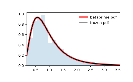
Display the probability density function (
pdf):>>> x = np.linspace(betaprime.ppf(0.01, a, b), ... betaprime.ppf(0.99, a, b), 100) >>> ax.plot(x, betaprime.pdf(x, a, b), ... 'r-', lw=5, alpha=0.6, label='betaprime pdf')
Alternatively, the distribution object can be called (as a function) to fix the shape, location and scale parameters. This returns a “frozen” RV object holding the given parameters fixed.
Freeze the distribution and display the frozen
pdf:>>> rv = betaprime(a, b) >>> ax.plot(x, rv.pdf(x), 'k-', lw=2, label='frozen pdf')
Check accuracy of
cdfandppf:>>> vals = betaprime.ppf([0.001, 0.5, 0.999], a, b) >>> np.allclose([0.001, 0.5, 0.999], betaprime.cdf(vals, a, b)) True
Generate random numbers:
>>> r = betaprime.rvs(a, b, size=1000)
And compare the histogram:
>>> ax.hist(r, density=True, bins='auto', histtype='stepfilled', alpha=0.2)
>>> ax.set_xlim([x[0], x[-1]])
>>> ax.legend(loc='best', frameon=False)
>>> plt.show()