scipy.stats.beta

scipy.stats.beta = <scipy.stats._continuous_distns.beta_gen object>

A beta continuous random variable.

As an instance of the rv_continuous class, beta object inherits from it a collection of generic methods (see below for the full list), and completes them with details specific for this particular distribution.

Methods

rvs(a, b, loc=0, scale=1, size=1, random_state=None)	Random variates.
pdf(x, a, b, loc=0, scale=1)	Probability density function.
logpdf(x, a, b, loc=0, scale=1)	Log of the probability density function.
cdf(x, a, b, loc=0, scale=1)	Cumulative distribution function.
logcdf(x, a, b, loc=0, scale=1)	Log of the cumulative distribution function.
sf(x, a, b, loc=0, scale=1)	Survival function (also defined as 1 - cdf, but sf is sometimes more accurate).
logsf(x, a, b, loc=0, scale=1)	Log of the survival function.
ppf(q, a, b, loc=0, scale=1)	Percent point function (inverse of cdf — percentiles).
isf(q, a, b, loc=0, scale=1)	Inverse survival function (inverse of sf).
moment(order, a, b, loc=0, scale=1)	Non-central moment of the specified order.
stats(a, b, loc=0, scale=1, moments=’mv’)	Mean(‘m’), variance(‘v’), skew(‘s’), and/or kurtosis(‘k’).
entropy(a, b, loc=0, scale=1)	(Differential) entropy of the RV.
fit(data)	Parameter estimates for generic data. See scipy.stats.rv_continuous.fit for detailed documentation of the keyword arguments.
expect(func, args=(a, b), loc=0, scale=1, lb=None, ub=None, conditional=False, **kwds)	Expected value of a function (of one argument) with respect to the distribution.
median(a, b, loc=0, scale=1)	Median of the distribution.
mean(a, b, loc=0, scale=1)	Mean of the distribution.
var(a, b, loc=0, scale=1)	Variance of the distribution.
std(a, b, loc=0, scale=1)	Standard deviation of the distribution.
interval(confidence, a, b, loc=0, scale=1)	Confidence interval with equal areas around the median.

Notes

The probability density function for beta is:

\[f(x, a, b) = \frac{\Gamma(a+b) x^{a-1} (1-x)^{b-1}} {\Gamma(a) \Gamma(b)}\]

for \(0 <= x <= 1\), \(a > 0\), \(b > 0\), where \(\Gamma\) is the gamma function (scipy.special.gamma).

beta takes \(a\) and \(b\) as shape parameters.

This distribution uses routines from the Boost Math C++ library for the computation of the pdf, cdf, ppf, sf and isf methods. [1]

Maximum likelihood estimates of parameters are only available when the location and scale are fixed. When either of these parameters is free, beta.fit resorts to numerical optimization, but this problem is unbounded: the location and scale may be chosen to make the minimum and maximum elements of the data coincide with the endpoints of the support, and the shape parameters may be chosen to make the PDF at these points infinite. For best results, pass floc and fscale keyword arguments to fix the location and scale, or use scipy.stats.fit with method='mse'.

The probability density above is defined in the “standardized” form. To shift and/or scale the distribution use the loc and scale parameters. Specifically, beta.pdf(x, a, b, loc, scale) is identically equivalent to beta.pdf(y, a, b) / scale with y = (x - loc) / scale. Note that shifting the location of a distribution does not make it a “noncentral” distribution; noncentral generalizations of some distributions are available in separate classes.

References

[1]

The Boost Developers. “Boost C++ Libraries”. https://www.boost.org/.

Examples

Try it in your browser!

>>> import numpy as np
>>> from scipy.stats import beta
>>> import matplotlib.pyplot as plt
>>> fig, ax = plt.subplots(1, 1)

Get the support:

>>> a, b = 2.31, 0.627
>>> lb, ub = beta.support(a, b)

Calculate the first four moments:

>>> mean, var, skew, kurt = beta.stats(a, b, moments='mvsk')

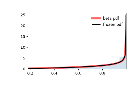
Display the probability density function (pdf):

>>> x = np.linspace(beta.ppf(0.01, a, b),
...                 beta.ppf(0.99, a, b), 100)
>>> ax.plot(x, beta.pdf(x, a, b),
...        'r-', lw=5, alpha=0.6, label='beta pdf')

Alternatively, the distribution object can be called (as a function) to fix the shape, location and scale parameters. This returns a “frozen” RV object holding the given parameters fixed.

Freeze the distribution and display the frozen pdf:

>>> rv = beta(a, b)
>>> ax.plot(x, rv.pdf(x), 'k-', lw=2, label='frozen pdf')

Check accuracy of cdf and ppf:

>>> vals = beta.ppf([0.001, 0.5, 0.999], a, b)
>>> np.allclose([0.001, 0.5, 0.999], beta.cdf(vals, a, b))
True

Generate random numbers:

>>> r = beta.rvs(a, b, size=1000)

And compare the histogram:

>>> ax.hist(r, density=True, bins='auto', histtype='stepfilled', alpha=0.2)
>>> ax.set_xlim([x[0], x[-1]])
>>> ax.legend(loc='best', frameon=False)
>>> plt.show()

Go BackOpen In Tab