scipy.special.

mathieu_odd_coef#

scipy.special.mathieu_odd_coef(m, q)[source]#

Fourier coefficients for odd Mathieu and modified Mathieu functions.

The Fourier series of the odd solutions of the Mathieu differential equation are of the form

\[\mathrm{se}_{2n+1}(z, q) = \sum_{k=0}^{\infty} B_{(2n+1)}^{(2k+1)} \sin (2k+1)z\]

\[\mathrm{se}_{2n+2}(z, q) = \sum_{k=0}^{\infty} B_{(2n+2)}^{(2k+2)} \sin (2k+2)z\]

This function returns the coefficients \(B_{(2n+2)}^{(2k+2)}\) for even input m=2n+2, and the coefficients \(B_{(2n+1)}^{(2k+1)}\) for odd input m=2n+1.

Parameters:

mint: Order of Mathieu functions. Must be non-negative.
qfloat (>=0): Parameter of Mathieu functions. Must be non-negative.

Returns:

Bkndarray: Even or odd Fourier coefficients, corresponding to even or odd m. The number of coefficients returned is determined by an empirical formula that depends on m and q [1].

See also

mathieu_sem
mathieu_even_coef

References

[1]

Zhang, Shanjie and Jin, Jianming. “Computation of Special Functions”, John Wiley and Sons, 1996. Original source code hosted by John Burkardt: https://people.sc.fsu.edu/~jburkardt/f77_src/special_functions/special_functions.html

[2]

NIST Digital Library of Mathematical Functions https://dlmf.nist.gov/28.4#i

Examples

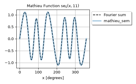
We use the Fourier coefficients to construct an approximation of mathieu_sem(5, 11, x), the odd Mathieu function of order m = 5 and parameter q = 11.

>>> import numpy as np
>>> import matplotlib.pyplot as plt
>>> from scipy.special import mathieu_odd_coef, mathieu_sem
>>> m = 5
>>> q = 11

b holds the Fourier coefficients. As noted above, the number of coefficients returned by mathieu_odd_coef(m, q) is based on an empirical formula that depends on m and q. In this case, we get 28 coefficients.

>>> b = mathieu_odd_coef(m, q)
>>> b.shape
(28,)

Sum the Fourier sine series on a grid of x values.

>>> period = 180 if m % 2 == 0 else 360
>>> x = np.linspace(0, period, 5000)               # x has shape (5000,)
>>> k = np.arange(1, len(b) + 1).reshape((-1, 1))  # k has shape (len(b), 1)
>>> c = np.sin((2*k - m % 2) * (np.pi/180) * x)    # c has shape (len(b), 5000)
>>> y = b @ c                                      # y has shape (5000,)

Plot the approximation, along with the function computed directly by mathieu_sem(m, q, x).

>>> plt.plot(x, y, 'k--', label="Fourier sum")
>>> se, _sce = mathieu_sem(m, q, x)
>>> plt.plot(x, se, alpha=0.35, linewidth=3.5, label="mathieu_sem")
>>> plt.grid(True)
>>> plt.title(f'Mathieu Function $\\rm{{se_{m}}}(x, {q})$')
>>> plt.xlabel('x [degrees]')
>>> plt.legend(shadow=True, loc='upper left', bbox_to_anchor=(1, 1))
>>> plt.tight_layout()
>>> plt.show()

../../_images/scipy-special-mathieu_odd_coef-1.png