scipy.special.eval_gegenbauer#

scipy.special.eval_gegenbauer(n, alpha, x, out=None) = <wrapped_ufunc 'eval_gegenbauer'>#

Evaluate Gegenbauer (ultraspherical) polynomial at a point.

The Gegenbauer polynomials can be defined via the Gauss hypergeometric function \({}_2F_1\) as

\[C_n^{(\alpha)}(x) = \frac{(2\alpha)_n}{\Gamma(n + 1)} {}_2F_1(-n, 2\alpha + n; \alpha + 1/2; (1 - x)/2).\]

where \((\cdot)_n\) is the Pochhammer symbol; see poch. When \(n\) is an integer the result is a polynomial of degree \(n\). See 22.5.46 in [AS] (or equivalently [DLMF]) for details.

Parameters:

narray_like: Degree of the polynomial. If not an integer, the result is determined via the relation to the Gauss hypergeometric function.
alphaarray_like: Parameter.
xarray_like: Points at which to evaluate the Gegenbauer polynomial.
outndarray, optional: Optional output array for the function values.

Returns:

Cscalar or ndarray: Values of the Gegenbauer polynomial.

See also

roots_gegenbauer: roots and quadrature weights of Gegenbauer polynomials
gegenbauer: Gegenbauer polynomial object
hyp2f1: Gauss hypergeometric function

Notes

Array API Standard Support

eval_gegenbauer has support for Python Array API Standard compatible backends in addition to NumPy. The following combinations of backend and device (or other capability) are supported.

Library	CPU	GPU
NumPy	✅	n/a
CuPy	n/a	⛔
PyTorch	✅	⛔
JAX	✅	⛔
Dask	✅	n/a

For the NumPy backend, this function supports all NumPy ufunc keyword arguments. Other backends may support out, but typically none of the other ufunc kwargs. out is typically supported for CuPy and PyTorch, but not currently in cases where SciPy relies on a generic Array API implementation or, for PyTorch on CPU, falls back to the NumPy backend. out is never supported for JAX because JAX arrays are immutable. eval_gegenbauer does not currently support out for the PyTorch backend.

See Support for the array API standard for more information.

References

[AS]

Milton Abramowitz and Irene A. Stegun, eds. Handbook of Mathematical Functions with Formulas, Graphs, and Mathematical Tables. New York: Dover, 1972.

[DLMF]

NIST Digital Library of Mathematical Functions, https://dlmf.nist.gov/18.5.E9

Examples

>>> import numpy as np
>>> from scipy.special import eval_gegenbauer
>>> import matplotlib.pyplot as plt

This is the parameter value that we’ll use in this example.

>>> alpha = 1.25

Evaluate the order 3 polynomial at a few values of x.

>>> eval_gegenbauer(3, alpha, [0, 0.25, 0.5])
array([ 0.        , -1.21582031, -1.2890625 ])

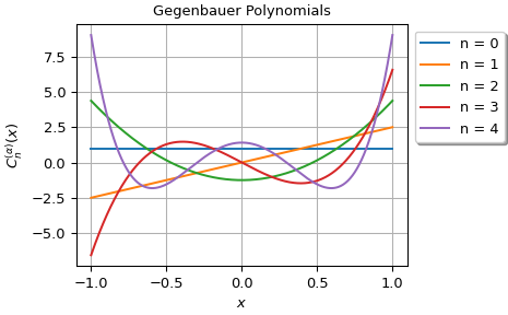
Plot the polynomials of order 0 through 4.

>>> x = np.linspace(-1, 1, 800)
>>> fig, ax = plt.subplots(1, 1, constrained_layout=True)
>>> for n in range(5):
...     y = eval_gegenbauer(n, alpha, x)
...     ax.plot(x, y, label=f'{n = }')
>>> ax.grid()
>>> ax.set_title("Gegenbauer Polynomials")
>>> ax.set_xlabel("$x$")
>>> ax.set_ylabel(r"$C_n^{(\alpha)}(x)$")
>>> ax.legend(loc='upper left', bbox_to_anchor=(1, 1), shadow=True)
>>> plt.show()

../../_images/scipy-special-eval_gegenbauer-1.png