scipy.signal.

square

scipy.signal.square(t, duty=0.5)

Return a periodic square-wave waveform.

The square wave has a period 2*pi, has value +1 from 0 to 2*pi*duty and -1 from 2*pi*duty to 2*pi. duty must be in the interval [0,1].

Note that this is not band-limited. It produces an infinite number of harmonics, which are aliased back and forth across the frequency spectrum.

Parameters:

tarray_like

The input time array.

dutyarray_like, optional

Duty cycle. Default is 0.5 (50% duty cycle). If an array, causes wave shape to change over time, and must be the same length as t.

Returns:

yndarray

Output array containing the square waveform.

Notes

Array API Standard Support

square has experimental support for Python Array API Standard compatible backends in addition to NumPy. Please consider testing these features by setting an environment variable SCIPY_ARRAY_API=1 and providing CuPy, PyTorch, JAX, or Dask arrays as array arguments. The following combinations of backend and device (or other capability) are supported.

Library	CPU	GPU
NumPy	✅	n/a
CuPy	n/a	⛔
PyTorch	⛔	⛔
JAX	⛔	⛔
Dask	⛔	n/a

See Support for the array API standard for more information.

Examples

Try it in your browser!

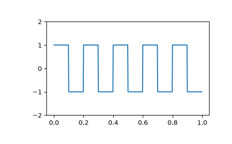
A 5 Hz waveform sampled at 500 Hz for 1 second:

>>> import numpy as np
>>> from scipy import signal
>>> import matplotlib.pyplot as plt
>>> t = np.linspace(0, 1, 500, endpoint=False)
>>> plt.plot(t, signal.square(2 * np.pi * 5 * t))
>>> plt.ylim(-2, 2)

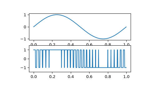
A pulse-width modulated sine wave:

>>> plt.figure()
>>> sig = np.sin(2 * np.pi * t)
>>> pwm = signal.square(2 * np.pi * 30 * t, duty=(sig + 1)/2)
>>> plt.subplot(2, 1, 1)
>>> plt.plot(t, sig)
>>> plt.subplot(2, 1, 2)
>>> plt.plot(t, pwm)
>>> plt.ylim(-1.5, 1.5)

Go BackOpen In Tab