scipy.signal.

periodogram#

scipy.signal.periodogram(x, fs=1.0, window='boxcar', nfft=None, detrend='constant', return_onesided=True, scaling='density', axis=-1)[source]#

Estimate power spectral density using a periodogram.

Parameters:

xarray_like: Time series of measurement values
fsfloat, optional: Sampling frequency of the x time series. Defaults to 1.0.
windowstr or tuple or array_like, optional: Desired window to use. If window is a string or tuple, it is passed to get_window to generate the window values, which are DFT-even by default. See get_window for a list of windows and required parameters. If window is array_like it will be used directly as the window and its length must be equal to the length of the axis over which the periodogram is computed. Defaults to ‘boxcar’.
nfftint, optional: Length of the FFT used. If None the length of x will be used.
detrendstr or function or False, optional: Specifies how to detrend each segment. If detrend is a string, it is passed as the type argument to the detrend function. If it is a function, it takes a segment and returns a detrended segment. If detrend is False, no detrending is done. Defaults to ‘constant’.
return_onesidedbool, optional: If True, return a one-sided spectrum for real data. If False return a two-sided spectrum. Defaults to True, but for complex data, a two-sided spectrum is always returned.
scaling{ ‘density’, ‘spectrum’ }, optional: Selects between computing the power spectral density (‘density’) where Pxx has units of V²/Hz and computing the squared magnitude spectrum (‘spectrum’) where Pxx has units of V², if x is measured in V and fs is measured in Hz. Defaults to ‘density’
axisint, optional: Axis along which the periodogram is computed; the default is over the last axis (i.e. axis=-1).

Returns:

fndarray: Array of sample frequencies.
Pxxndarray: Power spectral density or power spectrum of x.

See also

welch: Estimate power spectral density using Welch’s method
lombscargle: Lomb-Scargle periodogram for unevenly sampled data

Notes

The ratio of the squared magnitude (scaling='spectrum') divided by the spectral power density (scaling='density') is the constant factor of sum(abs(window)**2)*fs / abs(sum(window))**2. If return_onesided is True, the values of the negative frequencies are added to values of the corresponding positive ones.

Consult the Spectral Analysis section of the SciPy User Guide for a discussion of the scalings of the power spectral density and the magnitude (squared) spectrum.

Added in version 0.12.0.

Array API Standard Support

periodogram has experimental support for Python Array API Standard compatible backends in addition to NumPy. Please consider testing these features by setting an environment variable SCIPY_ARRAY_API=1 and providing CuPy, PyTorch, JAX, or Dask arrays as array arguments. The following combinations of backend and device (or other capability) are supported.

Library	CPU	GPU
NumPy	✅	n/a
CuPy	n/a	⛔
PyTorch	⛔	⛔
JAX	⛔	⛔
Dask	⛔	n/a

See Support for the array API standard for more information.

Examples

>>> import numpy as np
>>> from scipy import signal
>>> import matplotlib.pyplot as plt
>>> rng = np.random.default_rng()

Generate a test signal, a 2 Vrms sine wave at 1234 Hz, corrupted by 0.001 V**2/Hz of white noise sampled at 10 kHz.

>>> fs = 10e3
>>> N = 1e5
>>> amp = 2*np.sqrt(2)
>>> freq = 1234.0
>>> noise_power = 0.001 * fs / 2
>>> time = np.arange(N) / fs
>>> x = amp*np.sin(2*np.pi*freq*time)
>>> x += rng.normal(scale=np.sqrt(noise_power), size=time.shape)

Compute and plot the power spectral density.

>>> f, Pxx_den = signal.periodogram(x, fs)
>>> plt.semilogy(f, Pxx_den)
>>> plt.ylim([1e-7, 1e2])
>>> plt.xlabel('frequency [Hz]')
>>> plt.ylabel('PSD [V**2/Hz]')
>>> plt.show()

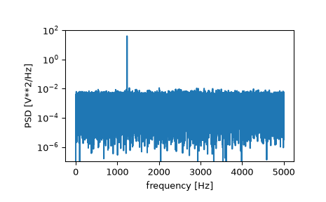
../../_images/scipy-signal-periodogram-1_00_00.png

If we average the last half of the spectral density, to exclude the peak, we can recover the noise power on the signal.

>>> np.mean(Pxx_den[25000:])
0.000985320699252543

Now compute and plot the power spectrum.

>>> f, Pxx_spec = signal.periodogram(x, fs, 'flattop', scaling='spectrum')
>>> plt.figure()
>>> plt.semilogy(f, np.sqrt(Pxx_spec))
>>> plt.ylim([1e-4, 1e1])
>>> plt.xlabel('frequency [Hz]')
>>> plt.ylabel('Linear spectrum [V RMS]')
>>> plt.show()

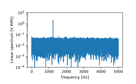
../../_images/scipy-signal-periodogram-1_01_00.png

The peak height in the power spectrum is an estimate of the RMS amplitude.

>>> np.sqrt(Pxx_spec.max())
2.0077340678640727