scipy.signal.

lp2hp#

scipy.signal.lp2hp(b, a, wo=1.0)[source]#

Transform a lowpass filter prototype to a highpass filter.

Return an analog high-pass filter with cutoff frequency wo from an analog low-pass filter prototype with unity cutoff frequency, in transfer function (‘ba’) representation.

Parameters:

barray_like: Numerator polynomial coefficients.
aarray_like: Denominator polynomial coefficients.
wofloat: Desired cutoff, as angular frequency (e.g., rad/s). Defaults to no change.

Returns:

barray_like: Numerator polynomial coefficients of the transformed high-pass filter.
aarray_like: Denominator polynomial coefficients of the transformed high-pass filter.

See also

lp2lp, lp2bp, lp2bs, bilinear
lp2hp_zpk

Notes

This is derived from the s-plane substitution

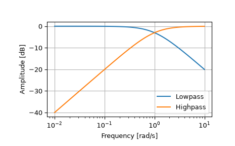
\[s \rightarrow \frac{\omega_0}{s}\]

This maintains symmetry of the lowpass and highpass responses on a logarithmic scale.

Array API Standard Support

lp2hp has experimental support for Python Array API Standard compatible backends in addition to NumPy. Please consider testing these features by setting an environment variable SCIPY_ARRAY_API=1 and providing CuPy, PyTorch, JAX, or Dask arrays as array arguments. The following combinations of backend and device (or other capability) are supported.

Library	CPU	GPU
NumPy	✅	n/a
CuPy	n/a	✅
PyTorch	✅	✅
JAX	⛔	⛔
Dask	⚠️ computes graph	n/a

See Support for the array API standard for more information.

Examples

>>> from scipy import signal
>>> import matplotlib.pyplot as plt

>>> lp = signal.lti([1.0], [1.0, 1.0])
>>> hp = signal.lti(*signal.lp2hp(lp.num, lp.den))
>>> w, mag_lp, p_lp = lp.bode()
>>> w, mag_hp, p_hp = hp.bode(w)

>>> plt.plot(w, mag_lp, label='Lowpass')
>>> plt.plot(w, mag_hp, label='Highpass')
>>> plt.semilogx()
>>> plt.grid(True)
>>> plt.xlabel('Frequency [rad/s]')
>>> plt.ylabel('Amplitude [dB]')
>>> plt.legend()