scipy.signal.

freqresp#

scipy.signal.freqresp(system, w=None, n=10000)[source]#

Calculate the frequency response of a continuous-time system.

Parameters:

systeman instance of the lti class or a tuple describing the system.

The following gives the number of elements in the tuple and the interpretation:

1 (instance of lti)

2 (num, den)

3 (zeros, poles, gain)

4 (A, B, C, D)

warray_like, optional

Array of frequencies (in rad/s). Magnitude and phase data is calculated for every value in this array. If not given, a reasonable set will be calculated.

nint, optional

Number of frequency points to compute if w is not given. The n frequencies are logarithmically spaced in an interval chosen to include the influence of the poles and zeros of the system.

Returns:

w1D ndarray: Frequency array [rad/s]
H1D ndarray: Array of complex magnitude values

Notes

If (num, den) is passed in for system, coefficients for both the numerator and denominator should be specified in descending exponent order (e.g. s^2 + 3s + 5 would be represented as [1, 3, 5]).

Array API Standard Support

freqresp has experimental support for Python Array API Standard compatible backends in addition to NumPy. Please consider testing these features by setting an environment variable SCIPY_ARRAY_API=1 and providing CuPy, PyTorch, JAX, or Dask arrays as array arguments. The following combinations of backend and device (or other capability) are supported.

Library	CPU	GPU
NumPy	✅	n/a
CuPy	n/a	⛔
PyTorch	⛔	⛔
JAX	⛔	⛔
Dask	⛔	n/a

See Support for the array API standard for more information.

Examples

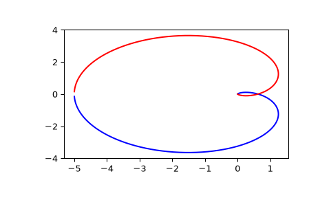
Generating the Nyquist plot of a transfer function

>>> from scipy import signal
>>> import matplotlib.pyplot as plt

Construct the transfer function \(H(s) = \frac{5}{(s-1)^3}\):

>>> s1 = signal.ZerosPolesGain([], [1, 1, 1], [5])

>>> w, H = signal.freqresp(s1)

>>> plt.figure()
>>> plt.plot(H.real, H.imag, "b")
>>> plt.plot(H.real, -H.imag, "r")
>>> plt.show()

../../_images/scipy-signal-freqresp-1.png