scipy.signal.dlti.

bode#

dlti.bode(w=None, n=100)[source]#

Calculate Bode magnitude and phase data of a discrete-time system.

Parameters:

warray_like, optional: Array of frequencies normalized to the Nyquist frequency being π, i.e., having unit radiant / sample. Magnitude and phase data is calculated for every value in this array. If not given, a reasonable set will be calculated.
nint, optional: Number of frequency points to compute if w is not given. The n frequencies are logarithmically spaced in an interval chosen to include the influence of the poles and zeros of the system. Defaults to 100.

Returns:

w1D ndarray: Array of frequencies normalized to the Nyquist frequency being np.pi/dt with dt being the sampling interval of the system parameter. The unit is rad/s assuming dt is in seconds.
mag1D ndarray: Magnitude array in dB
phase1D ndarray: Phase array in degrees

See also

Examples

>>> from scipy import signal
>>> import matplotlib.pyplot as plt

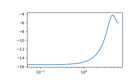
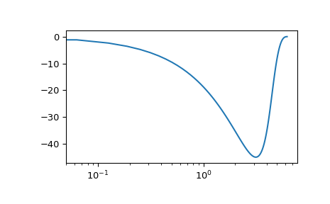
Construct the transfer function \(H(z) = \frac{1}{z^2 + 2z + 3}\) with sampling time 0.5s:

>>> sys = signal.TransferFunction([1], [1, 2, 3], dt=0.5)

Equivalent: signal.dbode(sys)

>>> w, mag, phase = sys.bode()

>>> plt.figure()
>>> plt.semilogx(w, mag)    # Bode magnitude plot
>>> plt.figure()
>>> plt.semilogx(w, phase)  # Bode phase plot
>>> plt.show()