scipy.signal.

cheb1ap

scipy.signal.cheb1ap(N, rp, *, xp=None, device=None)

Return (z, p, k) for Nth-order Chebyshev type I analog lowpass filter.

The returned filter prototype has rp decibels of ripple in the passband.

The filter’s angular (e.g. rad/s) cutoff frequency is normalized to 1, defined as the point at which the gain first drops below -rp.

Parameters:

Nint

The order of the filter

rpfloat

The passband ripple in dB. It constrains the passband gain to the interval [-rp, 0] dB.

xparray_namespace, optional

Optional array namespace. Should be compatible with the array API standard, or supported by array-api-compat. Default: numpy

deviceany

optional device specification for output. Should match one of the supported device specification in xp.

Returns:

zndarray[float64]

Zeros of the transfer function. Is always an empty array.

pndarray[complex128]

Poles of the transfer function.

kfloat

Gain of the transfer function.

See also

cheby1

Filter design function using this prototype

Notes

Array API Standard Support

cheb1ap has support for Python Array API Standard compatible backends in addition to NumPy. The following combinations of backend and device (or other capability) are supported.

Library	CPU	GPU
NumPy	✅	n/a
CuPy	n/a	✅
PyTorch	✅	✅
JAX	✅	✅
Dask	✅	n/a

See Support for the array API standard for more information.

Examples

Try it in your browser!

Compute the zeros, poles, and gain of a 3rd-order Chebyshev type I analog lowpass prototype with 1 dB of passband ripple:

>>> from scipy.signal import cheb1ap
>>> z, p, k = cheb1ap(3, 1)
>>> z
array([], dtype=float64)
>>> p
array([-0.2470853 +0.96599867j, -0.4941706 +0.j        ,
       -0.2470853 -0.96599867j])
>>> k
0.49130668209006784

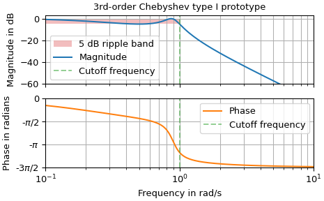
Plot of the frequency response of a 3rd-order prototype with a passband ripple of 5 dB:

>>> import numpy as np
>>> import matplotlib.pyplot as plt
>>> from scipy.signal import freqs_zpk, cheb1ap
...
>>> z, p, k = cheb1ap(3, rp=5)
>>> f = np.geomspace(1e-1, 1e1, 200)
>>> _, h = freqs_zpk(z, p, k, worN=f)
>>> h_db, h_ph = 20 * np.log10(np.abs(h)), np.unwrap(np.angle(h))
...
>>> _, (ax0, ax1) = plt.subplots(2, 1, sharex='all', constrained_layout=True)
>>> ax0.set(title='3rd-order Chebyshev type I prototype', ylim=(-60, 3),
...         ylabel='Magnitude in dB', yticks=[-60, -40, -20, 0])
>>> ax0.fill((0, 0, 1, 1), (0, -5, -5, 0), 'C3', alpha=.3, label="5 dB ripple band")
>>> ax0.semilogx(f, h_db, 'C0', label='Magnitude')
>>> ax1.set(ylabel="Phase in radians", xlabel="Frequency in rad/s",
...         yticks=np.pi*np.arange(-1.5, 0.5, 0.5), ylim=(-1.5*np.pi, 0),
...         yticklabels=[r'-3$\pi$/2', r'-$\pi$', r'-$\pi$/2', '0'],
...         xlim=(f[0], f[-1]))
>>> ax1.semilogx(f, h_ph, 'C1', label='Phase')
>>> for ax_ in (ax0, ax1):
...     ax_.axvline(1.0, color='C2', ls='--', alpha=.5, label='Cutoff frequency')
...     ax_.grid(True, which='both')
...     ax_.legend()
>>> plt.show()

Go BackOpen In Tab