scipy.signal.ShortTimeFFT.

spectrogram

ShortTimeFFT.spectrogram(x, y=None, detr=None, *, p0=None, p1=None, k_offset=0, padding='zeros', axis=-1)

Calculate spectrogram or cross-spectrogram.

The spectrogram is the absolute square of the STFT, i.e., it is abs(S[q,p])**2 for given S[q,p] and thus is always non-negative. For two STFTs Sx[q,p], Sy[q,p], the cross-spectrogram is defined as Sx[q,p] * np.conj(Sy[q,p]) and is complex-valued. This is a convenience function for calling stft / stft_detrend, hence all parameters are discussed there.

Parameters:

xnp.ndarray

The input signal as real or complex valued array. For complex values, the property fft_mode must be set to ‘twosided’ or ‘centered’.

ynp.ndarray

The second input signal of the same shape as x. If None, it is assumed to be x. For complex values, the property fft_mode must be set to ‘twosided’ or ‘centered’.

detr‘linear’ | ‘constant’ | Callable[[np.ndarray], np.ndarray] | None

If ‘constant’, the mean is subtracted, if set to “linear”, the linear trend is removed from each segment. This is achieved by calling detrend. If detr is a function with one parameter, detr is applied to each segment. For None (default), no trends are removed.

p0int | None

The first element of the range of slices to calculate. If None then it is set to p_min, which is the smallest possible slice.

p1int | None

The end of the array. If None then p_max(n) is used.

k_offsetint

Index of first sample (t = 0) in x.

padding‘zeros’ | ‘edge’ | ‘even’ | ‘odd’

Kind of values which are added, when the sliding window sticks out on either the lower or upper end of the input x. Zeros are added if the default ‘zeros’ is set. For ‘edge’ either the first or the last value of x is used. ‘even’ pads by reflecting the signal on the first or last sample and ‘odd’ additionally multiplies it with -1.

axisint

The axis of x over which to compute the STFT. If not given, the last axis is used.

Returns:

S_xynp.ndarray

A real-valued array with non-negative values is returned, if x is y or y is None. The dimension is always by one larger than of x. The last axis always represents the time slices of the spectrogram. axis defines the frequency axis (default second to last). E.g., for a one-dimensional x, a complex 2d array is returned, with axis 0 representing frequency and axis 1 the time slices.

See also

stft

Perform the short-time Fourier transform.

stft_detrend

STFT with a trend subtracted from each segment.

scipy.signal.ShortTimeFFT

Class this method belongs to.

Notes

The cross-spectrogram may be interpreted as the time-frequency analogon of the cross-spectral density (consult csd). The absolute square |Sxy|² of a cross-spectrogram Sxy divided by the spectrograms Sxx and Syy can be interpreted as a coherence spectrogram Cxy := abs(Sxy)**2 / (Sxx*Syy), which is the time-frequency analogon to coherence.

If the STFT is parametrized to be a unitary transform, i.e., utilitzing from_win_equals_dual, then the value of the scalar product, hence also the energy, is preserved.

Examples

Try it in your browser!

The following example shows the spectrogram of a square wave with varying frequency \(f_i(t)\) (marked by a green dashed line in the plot) sampled with 20 Hz. The utilized Gaussian window is 50 samples or 2.5 s long. For the ShortTimeFFT, the parameter mfft=800 (oversampling factor 16) and the hop interval of 2 in was chosen to produce a sufficient number of points.

The plot’s colormap is logarithmically scaled as the power spectral density is in dB. The time extent of the signal x is marked by vertical dashed lines, and the shaded areas mark the presence of border effects.

>>> import matplotlib.pyplot as plt
>>> import numpy as np
>>> from scipy.signal import square, ShortTimeFFT
>>> from scipy.signal.windows import gaussian
...
>>> T_x, N = 1 / 20, 1000  # 20 Hz sampling rate for 50 s signal
>>> t_x = np.arange(N) * T_x  # time indexes for signal
>>> f_i = 5e-3*(t_x - t_x[N // 3])**2 + 1  # varying frequency
>>> x = square(2*np.pi*np.cumsum(f_i)*T_x)  # the signal
...
>>> g_std = 12  # standard deviation for Gaussian window in samples
>>> win = gaussian(50, std=g_std, sym=True)  # symmetric Gaussian wind.
>>> SFT = ShortTimeFFT(win, hop=2, fs=1/T_x, mfft=800, scale_to='psd')
>>> Sx2 = SFT.spectrogram(x)  # calculate absolute square of STFT
...
>>> fig1, ax1 = plt.subplots(figsize=(6., 4.))  # enlarge plot a bit
>>> t_lo, t_hi = SFT.extent(N)[:2]  # time range of plot
>>> ax1.set_title(rf"Spectrogram ({SFT.m_num*SFT.T:g}$\,s$ Gaussian " +
...               rf"window, $\sigma_t={g_std*SFT.T:g}\,$s)")
>>> ax1.set(xlabel=f"Time $t$ in seconds ({SFT.p_num(N)} slices, " +
...                rf"$\Delta t = {SFT.delta_t:g}\,$s)",
...         ylabel=f"Freq. $f$ in Hz ({SFT.f_pts} bins, " +
...                rf"$\Delta f = {SFT.delta_f:g}\,$Hz)",
...         xlim=(t_lo, t_hi))
>>> Sx_dB = 10 * np.log10(np.fmax(Sx2, 1e-4))  # limit range to -40 dB
>>> im1 = ax1.imshow(Sx_dB, origin='lower', aspect='auto',
...                  extent=SFT.extent(N), cmap='magma')
>>> ax1.plot(t_x, f_i, 'g--', alpha=.5, label='$f_i(t)$')
>>> fig1.colorbar(im1, label='Power Spectral Density ' +
...                          r"$20\,\log_{10}|S_x(t, f)|$ in dB")
...
>>> # Shade areas where window slices stick out to the side:
>>> for t0_, t1_ in [(t_lo, SFT.lower_border_end[0] * SFT.T),
...                  (SFT.upper_border_begin(N)[0] * SFT.T, t_hi)]:
...     ax1.axvspan(t0_, t1_, color='w', linewidth=0, alpha=.3)
>>> for t_ in [0, N * SFT.T]:  # mark signal borders with vertical line
...     ax1.axvline(t_, color='c', linestyle='--', alpha=0.5)
>>> ax1.legend()
>>> fig1.tight_layout()
>>> plt.show()

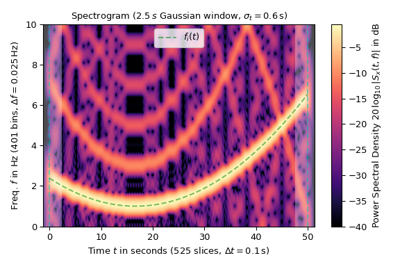
The logarithmic scaling reveals the odd harmonics of the square wave, which are reflected at the Nyquist frequency of 10 Hz. This aliasing is also the main source of the noise artifacts in the plot.

Go BackOpen In Tab