CZT#
- class scipy.signal.CZT(n, m=None, w=None, a=1 + 0j)[source]#
Create a callable chirp z-transform function.
Transform to compute the frequency response around a spiral. Objects of this class are callables which can compute the chirp z-transform on their inputs. This object precalculates the constant chirps used in the given transform.
- Parameters:
- nint
The size of the signal.
- mint, optional
The number of output points desired. Default is n.
- wcomplex, optional
The ratio between points in each step. This must be precise or the accumulated error will degrade the tail of the output sequence. Defaults to equally spaced points around the entire unit circle.
- acomplex, optional
The starting point in the complex plane. Default is 1+0j.
Methods
__call__(x, *[, axis])Calculate the chirp z-transform of a signal.
points()Return the points at which the chirp z-transform is computed.
- Returns:
- fCZT
Callable object
f(x, axis=-1)for computing the chirp z-transform on x.
See also
Notes
The defaults are chosen such that
f(x)is equivalent tofft.fft(x)and, ifm > len(x), thatf(x, m)is equivalent tofft.fft(x, m).If w does not lie on the unit circle, then the transform will be around a spiral with exponentially-increasing radius. Regardless, angle will increase linearly.
For transforms that do lie on the unit circle, accuracy is better when using
ZoomFFT, since any numerical error in w is accumulated for long data lengths, drifting away from the unit circle.The chirp z-transform can be faster than an equivalent FFT with zero padding. Try it with your own array sizes to see.
However, the chirp z-transform is considerably less precise than the equivalent zero-padded FFT.
As this CZT is implemented using the Bluestein algorithm, it can compute large prime-length Fourier transforms in O(N log N) time, rather than the O(N**2) time required by the direct DFT calculation. (
scipy.fftalso uses Bluestein’s algorithm’.)(The name “chirp z-transform” comes from the use of a chirp in the Bluestein algorithm. It does not decompose signals into chirps, like other transforms with “chirp” in the name.)
References
[1]Leo I. Bluestein, “A linear filtering approach to the computation of the discrete Fourier transform,” Northeast Electronics Research and Engineering Meeting Record 10, 218-219 (1968).
[2]Rabiner, Schafer, and Rader, “The chirp z-transform algorithm and its application,” Bell Syst. Tech. J. 48, 1249-1292 (1969).
Examples
Compute multiple prime-length FFTs:
>>> from scipy.signal import CZT
>>> import numpy as np
>>> a = np.random.rand(7)
>>> b = np.random.rand(7)
>>> c = np.random.rand(7)
>>> czt_7 = CZT(n=7)
>>> A = czt_7(a)
>>> B = czt_7(b)
>>> C = czt_7(c)
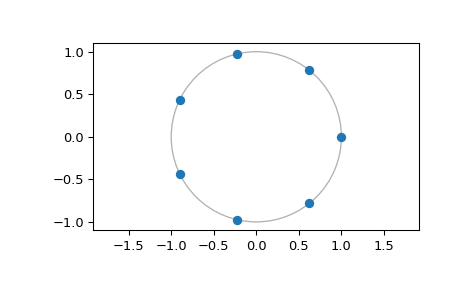
Display the points at which the FFT is calculated:
>>> czt_7.points()
array([ 1.00000000+0.j        ,  0.62348980+0.78183148j,
       -0.22252093+0.97492791j, -0.90096887+0.43388374j,
       -0.90096887-0.43388374j, -0.22252093-0.97492791j,
        0.62348980-0.78183148j])
>>> import matplotlib.pyplot as plt
>>> plt.plot(czt_7.points().real, czt_7.points().imag, 'o')
>>> plt.gca().add_patch(plt.Circle((0,0), radius=1, fill=False, alpha=.3))
>>> plt.axis('equal')
>>> plt.show()