scipy.signal.

czt#

scipy.signal.czt(x, m=None, w=None, a=1 + 0j, *, axis=-1)[source]#

Compute the frequency response around a spiral in the Z plane.

Parameters:

xarray: The signal to transform.
mint, optional: The number of output points desired. Default is the length of the input data.
wcomplex, optional: The ratio between points in each step. This must be precise or the accumulated error will degrade the tail of the output sequence. Defaults to equally spaced points around the entire unit circle.
acomplex, optional: The starting point in the complex plane. Default is 1+0j.
axisint, optional: Axis over which to compute the FFT. If not given, the last axis is used.

Returns:

outndarray: An array of the same dimensions as x, but with the length of the transformed axis set to m.

See also

CZT: Class that creates a callable chirp z-transform function.
zoom_fft: Convenience function for partial FFT calculations.

Notes

The defaults are chosen such that signal.czt(x) is equivalent to fft.fft(x) and, if m > len(x), that signal.czt(x, m) is equivalent to fft.fft(x, m).

If the transform needs to be repeated, use CZT to construct a specialized transform function which can be reused without recomputing constants.

An example application is in system identification, repeatedly evaluating small slices of the z-transform of a system, around where a pole is expected to exist, to refine the estimate of the pole’s true location. [1]

References

[1]

Steve Alan Shilling, “A study of the chirp z-transform and its applications”, pg 20 (1970) https://krex.k-state.edu/dspace/bitstream/handle/2097/7844/LD2668R41972S43.pdf

Examples

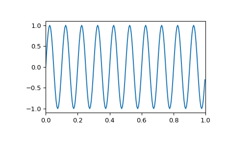
Generate a sinusoid:

>>> import numpy as np
>>> f1, f2, fs = 8, 10, 200  # Hz
>>> t = np.linspace(0, 1, fs, endpoint=False)
>>> x = np.sin(2*np.pi*t*f2)
>>> import matplotlib.pyplot as plt
>>> plt.plot(t, x)
>>> plt.axis([0, 1, -1.1, 1.1])
>>> plt.show()

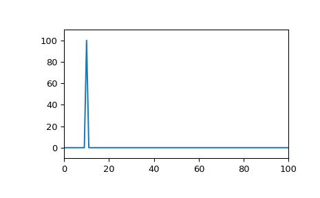
Its discrete Fourier transform has all of its energy in a single frequency bin:

>>> from scipy.fft import rfft, rfftfreq
>>> from scipy.signal import czt, czt_points
>>> plt.plot(rfftfreq(fs, 1/fs), abs(rfft(x)))
>>> plt.margins(0, 0.1)
>>> plt.show()

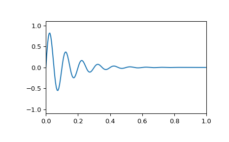
However, if the sinusoid is logarithmically-decaying:

>>> x = np.exp(-t*f1) * np.sin(2*np.pi*t*f2)
>>> plt.plot(t, x)
>>> plt.axis([0, 1, -1.1, 1.1])
>>> plt.show()

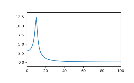
the DFT will have spectral leakage:

>>> plt.plot(rfftfreq(fs, 1/fs), abs(rfft(x)))
>>> plt.margins(0, 0.1)
>>> plt.show()

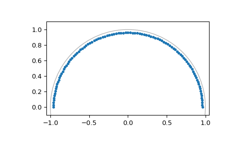
While the DFT always samples the z-transform around the unit circle, the chirp z-transform allows us to sample the Z-transform along any logarithmic spiral, such as a circle with radius smaller than unity:

>>> M = fs // 2  # Just positive frequencies, like rfft
>>> a = np.exp(-f1/fs)  # Starting point of the circle, radius < 1
>>> w = np.exp(-1j*np.pi/M)  # "Step size" of circle
>>> points = czt_points(M + 1, w, a)  # M + 1 to include Nyquist
>>> plt.plot(points.real, points.imag, '.')
>>> plt.gca().add_patch(plt.Circle((0,0), radius=1, fill=False, alpha=.3))
>>> plt.axis('equal'); plt.axis([-1.05, 1.05, -0.05, 1.05])
>>> plt.show()

With the correct radius, this transforms the decaying sinusoid (and others with the same decay rate) without spectral leakage:

>>> z_vals = czt(x, M + 1, w, a)  # Include Nyquist for comparison to rfft
>>> freqs = np.angle(points)*fs/(2*np.pi)  # angle = omega, radius = sigma
>>> plt.plot(freqs, abs(z_vals))
>>> plt.margins(0, 0.1)
>>> plt.show()